5.4 Titles and labels

We’ve been using the labs(tag = ) function to add tags to plots. But the labs() function can also be used to modify axis labels, or to add a title, subtitle, or a caption to your plot (Figure 5.7):

p13 <- p0 +
  labs(x = "Gross domestic product per capita",
       y = "Life expectancy",
       title = "Health and economics",
       subtitle = "Gapminder dataset, 2007",
       caption = Sys.Date(),
       tag = "p13")

p13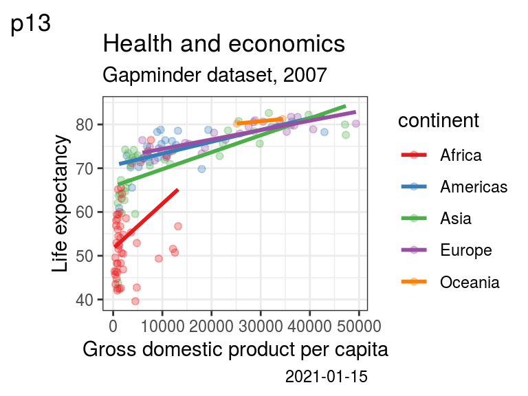

FIGURE 5.7: p13: Adding on a title, subtitle, caption using labs().

5.4.1 Annotation

In the previous chapter, we showed how use geom_text() and geom_label() to add text elements to a plot. Using geoms make sense when the values are based on data and variables mapped in aes(). They are efficient for including multiple pieces of text or labels on your data. For ‘hand’ annotating a plot, the annotate() function makes more sense, as you can quickly insert the type, location and label of your annotation (Figure 5.8):

p14 <- p0 +
  annotate("text",
           x = 25000,
           y = 50,
           label = "No points here!")

p15 <- p0 +
  annotate("label",
           x = 25000,
           y = 50,
           label = "No points here!")

p16 <- p0 +
  annotate("label",
           x = 25000, 
           y = 50,
           label = "No points here!", 
           hjust = 0)

p14 + labs(tag = "p14") + (p15 + labs(tag = "p15"))/ (p16 + labs(tag = "p16"))

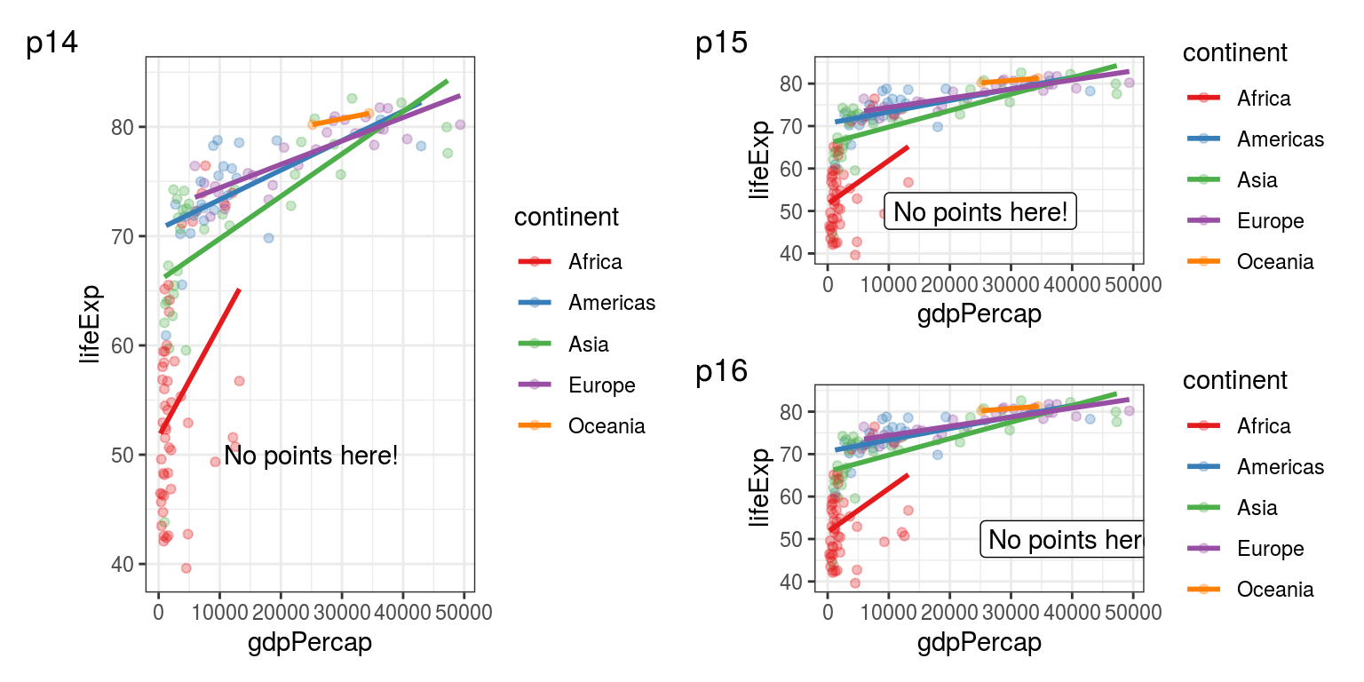
FIGURE 5.8: p14: annotate("text", ...) to quickly add a text on your plot. p15: annotate("label") is similar but draws a box around your text (making it a label). p16: Using hjust to control the horizontal justification of the annotation.

hjust stands for horizontal justification. Its default value is 0.5 (see how the label was centred at 25,000 - our chosen x location), 0 means the label goes to the right from 25,000, 1 would make it end at 25,000.

5.4.2 Annotation with a superscript and a variable

This is an advanced example on how to annotate your plot with something that has a superscipt and is based on a single value read in from a variable (Figure 5.9):

# a value we made up for this example
# a real analysis would get it from the linear model object
fit_glance <- tibble(r.squared = 0.7693465)


plot_rsquared <- paste0(
  "R^2 == ",
  fit_glance$r.squared %>% round(2))


p17 <- p0 +
  annotate("text",
           x = 25000, 
           y = 50,
           label = plot_rsquared, parse = TRUE,
           hjust = 0)

p17 + labs(tag = "p17")

FIGURE 5.9: p17: Using a superscript in your plot annotation.