5.5 Overall look - theme()

And finally, everything else on a plot - from font to background to the space between facets, can be changed using the theme() function. As you saw in the previous chapter, in addition to its default grey background, ggplot2 also comes with a few built-in themes, namely, theme_bw() or theme_classic(). These produce good looking plots that may already be publication ready. But if we do decide to tweak them, then the main theme() arguments we use are axis.text, axis.title, and legend.position.¹³ Note that all of these go inside the theme(), and that the axis.text and axis.title arguments are usually followed by = element_text() as shown in the examples below.

5.5.1 Text size

The way the axis.text and axis.title arguments of theme() work is that if you specify .x or .y it gets applied on that axis alone. But not specifying these, applies the change on both. Both the angle and vjust (vertical justification) options can be useful if your axis text doesn’t fit well and overlaps. It doesn’t usually make sense to change the colour of the font to anything other than "black", we are using green and red here to indicate which parts of the plot get changed with each line (Figure 5.10).

p18 <-  p0 +
  theme(axis.text.y = element_text(colour = "green", size = 14),
        axis.text.x = element_text(colour = "red",  angle = 45, vjust = 0.5),
        axis.title  = element_text(colour = "blue", size = 16)
        )

p18 + labs(tag = "p18")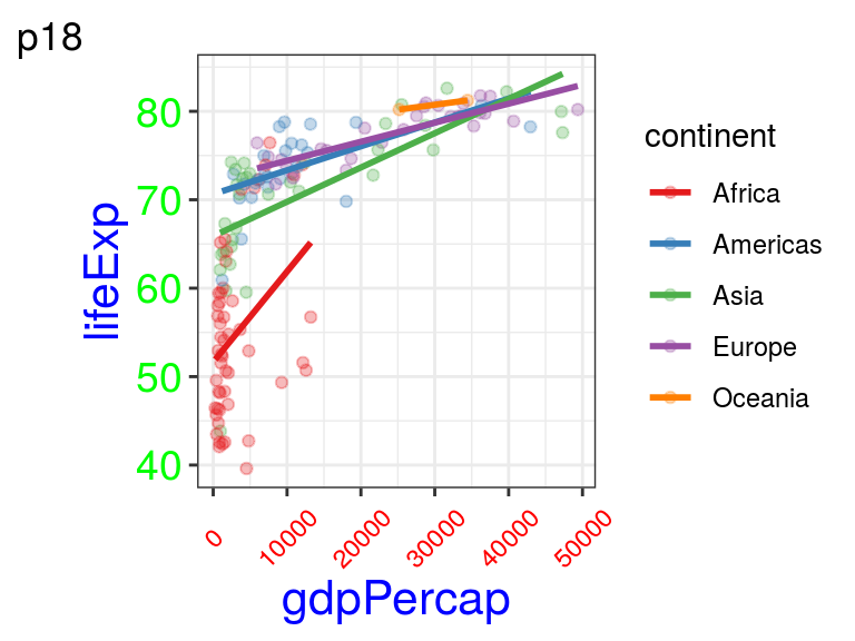

FIGURE 5.10: p18: Using axis.text and axis.title within theme() to tweak the appearance of your plot, including font size and angle. Coloured font is used to indicate which part of the code was used to change each element.

5.5.2 Legend position

The position of the legend can be changed using the legend.position argument within theme(). It can be positioned using the following words: "right", "left", "top", "bottom". Or to remove the legend completely, use "none":

p19 <- p0 +
  theme(legend.position = "none")

Alternatively, we can use relative coordinates (0–1) to give the legend a relative x-y location (Figure 5.11):

p20 <- p0 +
  theme(legend.position      = c(1,0), #bottom-right corner
        legend.justification = c(1,0)) 

p19 + labs(tag = "p19") + p20 + labs(tag = "p20")

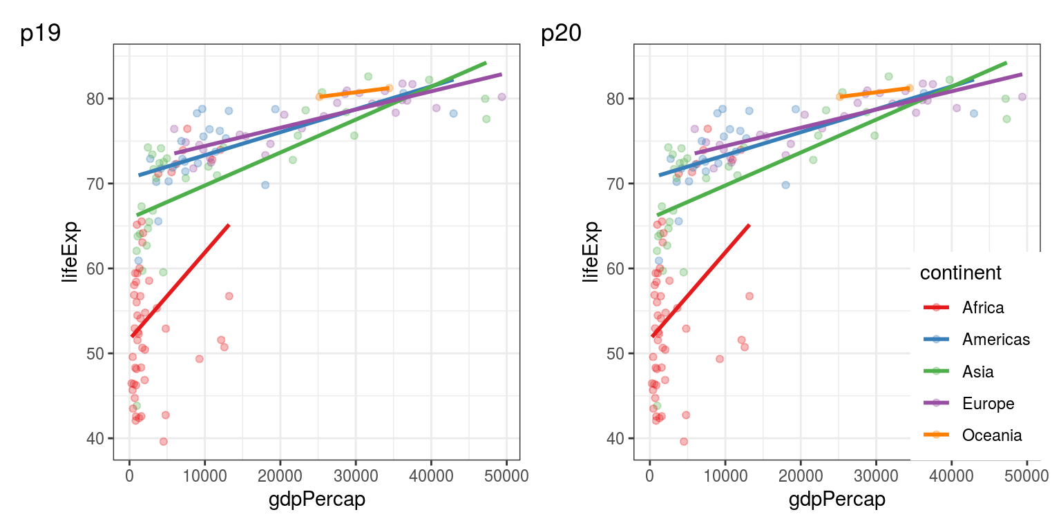
FIGURE 5.11: p19: Setting theme(legend.position = "none") removes it. p20: Relative coordinates such as theme(legend.position = c(1,0) can by used to place the legend within the plot area.

Further theme(legend.) options can be used to change the size, background, spacing, etc., of the legend. However, for modifying the content of the legend, you’ll have to use the guides() function. Again, ggplot()’s defaults are very good, and we rarely need to go into this much tweaking using both the theme() and guides() functions. But it is good to know what is possible.

For example, this is how to change the number of columns within the legend (Figure 5.12):

p21 <- p0 +
  guides(colour = guide_legend(ncol = 2)) +
  theme(legend.position = "top") # moving to the top optional

p21 + labs(tag = "p21")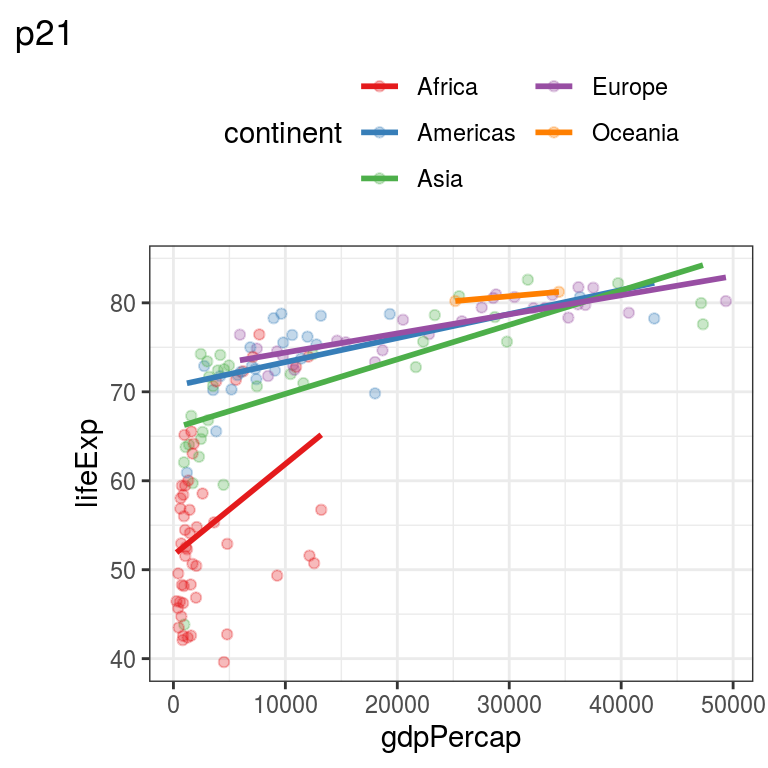

FIGURE 5.12: p21: Changing the number of columns within a legend.

---

13. To see a full list of possible arguments to theme(), navigate to it in the Help tab or find its online documentation at https://ggplot2.tidyverse.org/.↩︎