12.5 The anatomy of a Notebook / R Markdown file
When you create a file, a helpful template is provided to get you started.
Figure 12.3 shows the essential elements of a Notebook file and how these translate to the HTML preview.
12.5.1 YAML header
Every Notebook and Markdown file requires a “YAML header”. Where do they get these terms you ask? Originally YAML was said to mean Yet Another Markup Language, referencing its purpose as a markup language. It was later repurposed as YAML Ain’t Markup Language, a recursive acronym, to distinguish its purpose as data-oriented rather than document markup (thank you Wikipedia).
This is simply where many of the settings/options for file creation are placed. In RStudio, these often update automatically as different settings are invoked in the Options menu.
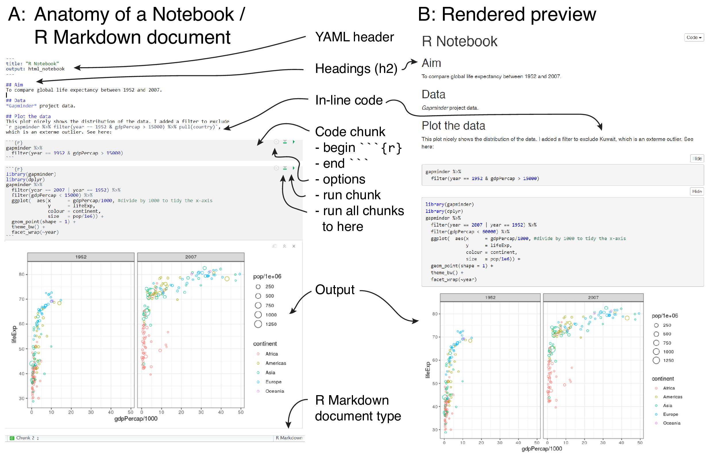
FIGURE 12.3: The Anatomy of a Notebook/Markdown file. Input (left) and output (right).
12.5.2 R code chunks
R code within a Notebook or Markdown file can be included in two ways:
- in-line: e.g., the total number of oranges was
`rsum(fruit$oranges)`; - as a “chunk”.
R chunks are flexible, come with lots of options, and you will soon get into the way of using them.
Figure 12.3 shows how a chunk fits into the document.
```{r}
# This is basic chunk.
# It always starts with ```{r}
# And ends with ```
# Code goes here
sum(fruit$oranges)
```
This may look off-putting, but just go with it for now.
You can type the four back-ticks in manually, or use the Insert button and choose R.
You will also notice that chunks are not limited to R code.
It is particularly helpful that Python can also be run in this way.
When doing an analysis in a Notebook you will almost always want to see the code and the output.
When you are creating a final document you may wish to hide code.
Chunk behaviour can be controlled via the Chunk Cog on the right of the chunk (Figure 12.3).
Table 12.1 shows the various permutations of code and output options that are available. The code is placed in the chunk header but the options fly-out now does this automatically, e.g.,
| Option | Code |
|---|---|
| Show output only | echo=FALSE |
| Show code and output | echo=TRUE |
| Show code (don’t run code) | eval=FALSE |
| Show nothing (run code) | include=FALSE |
| Show nothing (don’t run code) | include=FALSE, eval=FALSE |
| Hide warnings | warnings=FALSE |
| Hide messages | messages=FALSE |
12.5.3 Setting default chunk options
We can set default options for all our chunks at the top of our document by adding and editing knitr::opts_chunk$set(echo = TRUE) at the top of the document.
12.5.4 Setting default figure options
It is possible to set different default sizes for different output types by including these in the YAML header (or using the document cog):
---
title: "R Notebook"
output:
  pdf_document:
    fig_height: 3
    fig_width: 4
  html_document:
    fig_height: 6
    fig_width: 9
---
The YAML header is very sensitive to the spaces/tabs, so make sure these are correct.
12.5.5 Markdown elements
Markdown text can be included as you wish around your chunks. Figure 12.3 shows an example of how this can be done. This is a great way of getting into the habit of explicitly documenting your analysis. When you come back to a file in 6 months’ time, all of your thinking is there in front of you, rather than having to work out what on Earth you were on about from a collection of random code!