4.12 Extra: Advanced examples
There are two examples of how just a few lines of ggplot() code and the basic geoms introduced in this chapter can be used to make very different things.
Let your imagination fly free when using ggplot()!
Figure 4.18 shows how the life expectancies in European countries have increased by plotting a square (geom_point(shape = 15)) for each observation (year) in the dataset.
gapdata %>%
  filter(continent == "Europe") %>%
  ggplot(aes(y      = fct_reorder(country, lifeExp, .fun=max),
             x      = lifeExp,
             colour = year)) +
  geom_point(shape = 15, size = 2) +
  scale_colour_distiller(palette = "Greens", direction = 1) +
  theme_bw()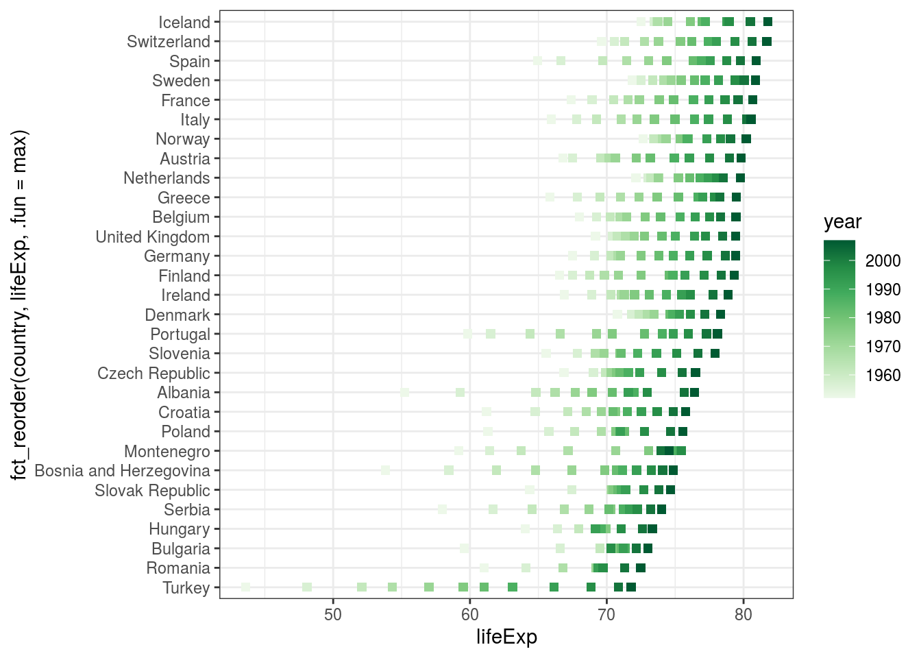
FIGURE 4.18: Increase in European life expectancies over time. Using fct_reorder() to order the countries on the y-axis by life expectancy (rather than alphabetically which is the default).
In Figure 4.19, we’re using group_by(continent) followed by mutate(country_number = seq_along(country)) to create a new column with numbers 1, 2, 3, etc., for countries within continents.
We are then using these as y coordinates for the text labels (geom_text(aes(y = country_number...).
gapdata2007 %>%
  group_by(continent) %>%
  mutate(country_number = seq_along(country)) %>%
  ggplot(aes(x = continent)) +
  geom_bar(aes(colour = continent), fill = NA, show.legend = FALSE) +
  geom_text(aes(y = country_number, label = country), vjust = 1)+
  geom_label(aes(label = continent), y = -1) +
  theme_void()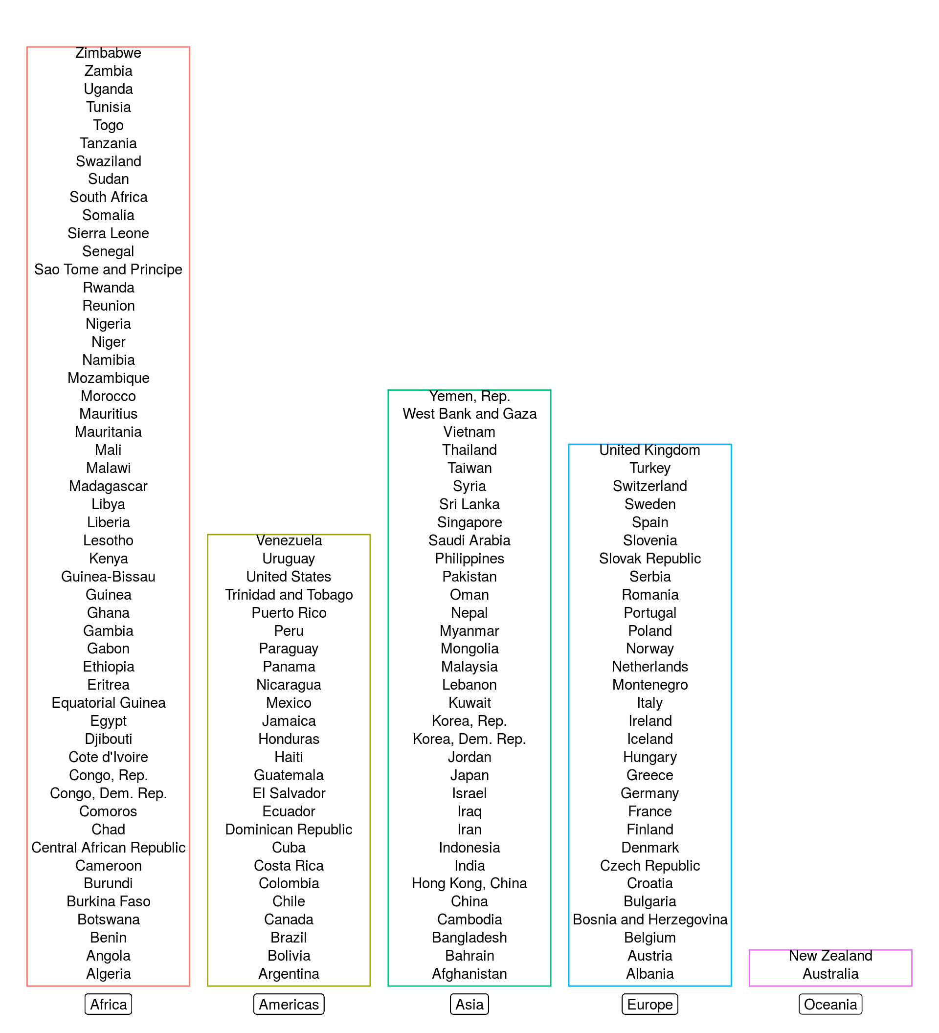
FIGURE 4.19: List of countries on each continent as in the gapminder dataset.