5.3 Colours

5.3.1 Using the Brewer palettes:

The easiest way to change the colour palette of your ggplot() is to specify a Brewer palette (Harrower and Brewer (2003)):

p9 <- p0 +
  scale_color_brewer(palette = "Paired")

Note that http://colorbrewer2.org/ also has options for Colourblind safe and Print friendly.

5.3.2 Legend title

scale_colour_brewer() is also a convenient place to change the legend title (Figure 5.5):

p10 <- p0 +
  scale_color_brewer("Continent - \n one of 5", palette = "Paired")

Note the \n inside the new legend title - new line.

p9 + labs(tag = "p9") + p10 + labs(tag = "p10")

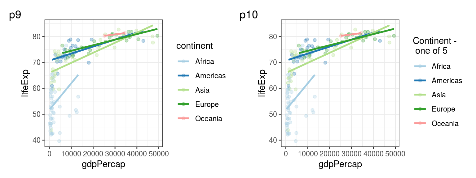
FIGURE 5.5: p9: Choosing a Brewer palette for your colours. p10: Changing the legend title.

5.3.3 Choosing colours manually

R also knows the names of many colours, so we can use words to specify colours:

p11 <- p0 +
  scale_color_manual(values = c("red", "green", "blue", "purple", "pink"))

The same function can also be used to use HEX codes for specifying colours:

p12 <- p0 +
  scale_color_manual(values = c("#8dd3c7", "#ffffb3", "#bebada",
                                "#fb8072", "#80b1d3"))

p11 + labs(tag = "p11") + p12 + labs(tag = "p12")

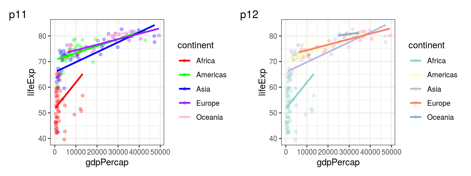
FIGURE 5.6: Colours can also be specified using words ("red", "green", etc.), or HEX codes ("#8dd3c7", "#ffffb3", etc.).

References

Harrower, Mark, and Cynthia A. Brewer. 2003. “ColorBrewer.org: An Online Tool for Selecting Colour Schemes for Maps.” The Cartographic Journal 40 (1): 27–37. https://doi.org/10.1179/000870403235002042.