2.1 Reading data into R
Data usually comes in the form of a table, such as a spreadsheet or database.
In the world of the tidyverse, a table read into R gets called a tibble.
A common format in which to receive data is CSV (comma separated values). CSV is an uncomplicated spreadsheet with no formatting. It is just a single table with rows and columns (no worksheets or formulas). Furthermore, you don’t need special software to quickly view a CSV file - a text editor will do, and that includes RStudio.
For example, look at “example_data.csv” in the healthyr project’s folder in Figure 2.1 (this is the Files pane at the bottom-right corner of your RStudio).
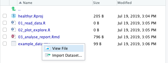
FIGURE 2.1: View or import a data file.
Clicking on a data file gives us two options: “View File” or “Import Dataset”.
We will show you how to use the Import Dataset interface in a bit, but for standard CSV files, we don’t usually bother with the Import interface and just type in (or copy from a previous script):
There are a couple of things to say about the first R code chunk of this book. First and foremost: do not panic. Yes, if you’re used to interacting with data by double-clicking on a spreadsheet that just opens up, then the above R code does seem a bit involved.
However, running the example above also has an immediate visual effect. As soon as you click Run (or press Ctrl+Enter/Command+Enter), the dataset immediately shows up in your Environment and opens in a Viewer. You can have a look and scroll through the same way you would in Excel or similar.
So what’s actually going on in the R code above:
- We load the tidyverse packages (as covered in the first chapter of this book).
- We have a CSV file called “example_data.csv” and are using
read_csv()to read it into R. - We are using the assignment arrow
<-to save it into our Environment using the same name:example_data. - The
View(example_data)line makes it pop up for us to view it. Alternatively, click onexample_datain the Environment to achieve the exact same thing.
More about the assignment arrow (<-) and naming things in R are covered later in this chapter.
Do not worry if everything is not crystal clear just now.
2.1.1 Import Dataset interface
In the read_csv() example above, we read in a file that was in a specific (but common) format.
However, if your file uses semicolons instead of commas, or commas instead of dots, or a special number for missing values (e.g., 99), or anything else weird or complicated, then we need a different approach.
RStudio’s Import Dataset interface (Figure 2.1) can handle all of these and more.
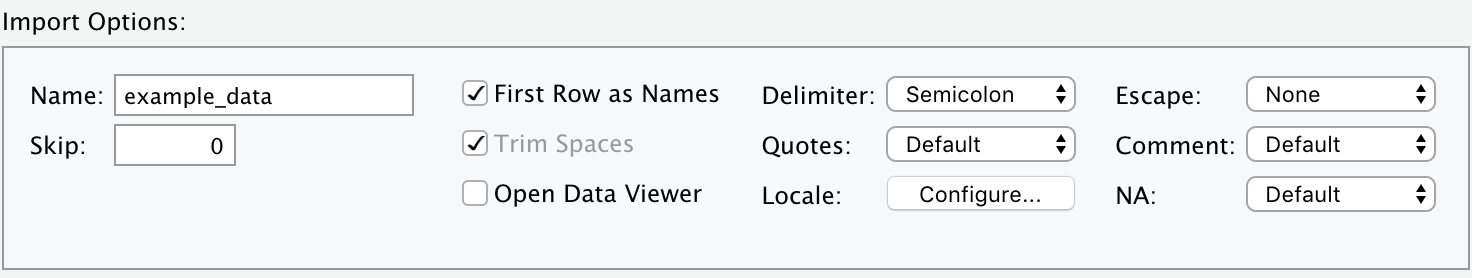
FIGURE 2.2: Import: Some of the special settings your data file might have.
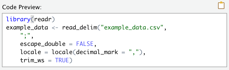
FIGURE 2.3: After using the Import Dataset window, copy-paste the resulting code into your script.
After selecting the specific options to import a particular file, a friendly preview window will show whether R properly understands the format of your data.
DO NOT BE tempted to press the Import button.
Yes, this will read in your dataset once, but means you have to reselect the options every time you come back to RStudio. Instead, copy-paste the code (e.g., Figure 2.3) into your R script. This way you can use it over and over again.
Ensuring that all steps of an analysis are recorded in scripts makes your workflow reproducible by your future self, colleagues, supervisors, and extraterrestrials.
The
Import Datasetbutton can also help you to read in Excel, SPSS, Stata, or SAS files (instead ofread_csv(), it will give youread_excel(),read_sav(),read_stata(), orread_sas()).
If you’ve used R before or are using older scripts passed by colleagues, you might see read.csv() rather than read_csv().
Note the dot rather than the underscore.
In short, read_csv() is faster and more predictable and in all new scripts is to be recommended.
In existing scripts that work and are tested, we do not recommend that you start replacing read.csv() with read_csv().
For instance, read_csv() handles categorical variables differently.2
An R script written using the read.csv() might not work as expected any more if just replaced with read_csv().
Do not start updating and possibly breaking existing R scripts by replacing base R functions with the tidyverse equivalents we show here. Do use the modern functions in any new code you write.
2.1.2 Reading in the Global Burden of Disease example dataset
In the next few chapters of this book, we will be using the Global Burden of Disease datasets. The Global Burden of Disease Study (GBD) is the most comprehensive worldwide observational epidemiological study to date. It describes mortality and morbidity from major diseases, injuries and risk factors to health at global, national and regional levels.3
GBD data are publicly available from the website.
Table 2.1 and Figure 2.4 show a high level version of the project data with just 3 variables: cause, year, deaths_millions (number of people who die of each cause every year).
Later, we will be using a longer dataset with different subgroups and we will show you how to summarise comprehensive datasets yourself.
| year | cause | deaths_millions |
|---|---|---|
| 1990 | Communicable diseases | 15.36 |
| 1990 | Injuries | 4.25 |
| 1990 | Non-communicable diseases | 26.71 |
| 1995 | Communicable diseases | 15.11 |
| 1995 | Injuries | 4.53 |
| 1995 | Non-communicable diseases | 29.27 |
| 2000 | Communicable diseases | 14.81 |
| 2000 | Injuries | 4.56 |
| 2000 | Non-communicable diseases | 31.01 |
| 2005 | Communicable diseases | 13.89 |
| 2005 | Injuries | 4.49 |
| 2005 | Non-communicable diseases | 32.87 |
| 2010 | Communicable diseases | 12.51 |
| 2010 | Injuries | 4.69 |
| 2010 | Non-communicable diseases | 35.43 |
| 2015 | Communicable diseases | 10.88 |
| 2015 | Injuries | 4.46 |
| 2015 | Non-communicable diseases | 39.28 |
| 2017 | Communicable diseases | 10.38 |
| 2017 | Injuries | 4.47 |
| 2017 | Non-communicable diseases | 40.89 |
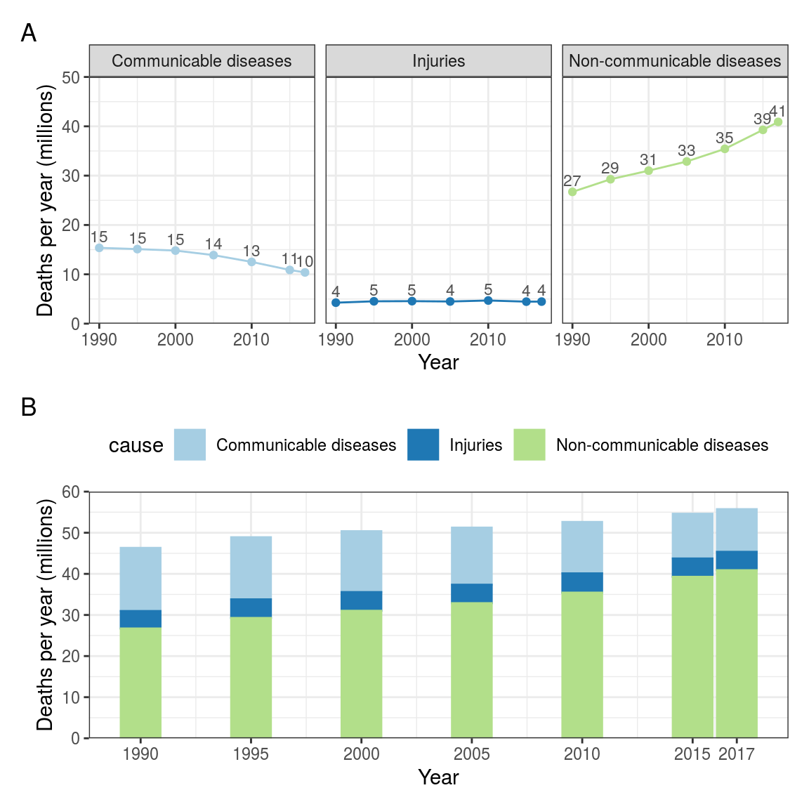
FIGURE 2.4: Line and bar charts: Cause of death by year (GBD). Data in (B) are the same as (A) but stacked to show the total of all causes.
It does not silently convert strings to factors, i.e., it defaults to
stringsAsFactors = FALSE. For those not familiar with the terminology here - don’t worry, we will cover this in just a few sections.↩︎Global Burden of Disease Collaborative Network. Global Burden of Disease Study 2017 (GBD 2017) Results. Seattle, United States: Institute for Health Metrics and Evaluation (IHME), 2018. Available from http://ghdx.healthdata.org/gbd-results-tool.↩︎