4.6 Bar plots
There are two geoms for making bar plots - geom_col() and geom_bar() and the examples below will illustrate when to use which one.
In short: if your data is already summarised or includes values for y (height of the bars), use geom_col().
If, however, you want ggplot() to count up the number of rows in your dataset, use geom_bar().
For example, with patient-level data (each row is a patient) you’ll probably want to use geom_bar(), with data that is already somewhat aggregated, you’ll use geom_col().
There is no harm in trying one, and if it doesn’t work, trying the other.
4.6.1 Summarised data
geom_col()requires two variablesaes(x = , y = )xis categorical,yis continuous (numeric)
Let’s plot the life expectancies in 2007 in these three countries:
gapdata2007 %>%
  filter(country %in% c("United Kingdom", "France", "Germany")) %>%
  ggplot(aes(x = country, y = lifeExp)) +
  geom_col()
This gives us Figure 4.10:1. We have also created another cheeky one using the same code but changing the scale of the y axis to be more dramatic (Figure 4.10:2).
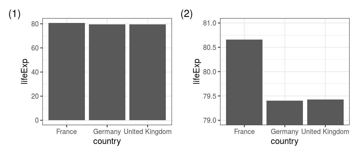
FIGURE 4.10: Bar plots using geom_col(): (1) using the code example, (2) same plot but with + coord_cartesian(ylim=c(79, 81)) to manipulate the scale into something a lot more dramatic.
4.6.2 Countable data
geom_bar()requires a single variableaes(x = )- this
xshould be a categorical variable geom_bar()then counts up the number of observations (rows) for this variable and plots them as bars.
Our gapdata2007 tibble has a row for each country (see end of Section 4.1 to remind yourself).
Therefore, if we use the count() function on the continent variable, we are counting up the number of countries on each continent (in this dataset12):
## # A tibble: 5 x 2
##   continent     n
##   <fct>     <int>
## 1 Africa       52
## 2 Americas     25
## 3 Asia         33
## 4 Europe       30
## 5 Oceania       2
So geom_bar() basically runs the count() function and plots it (see how the bars on Figure 4.11 are the same height as the values from count(continent)).
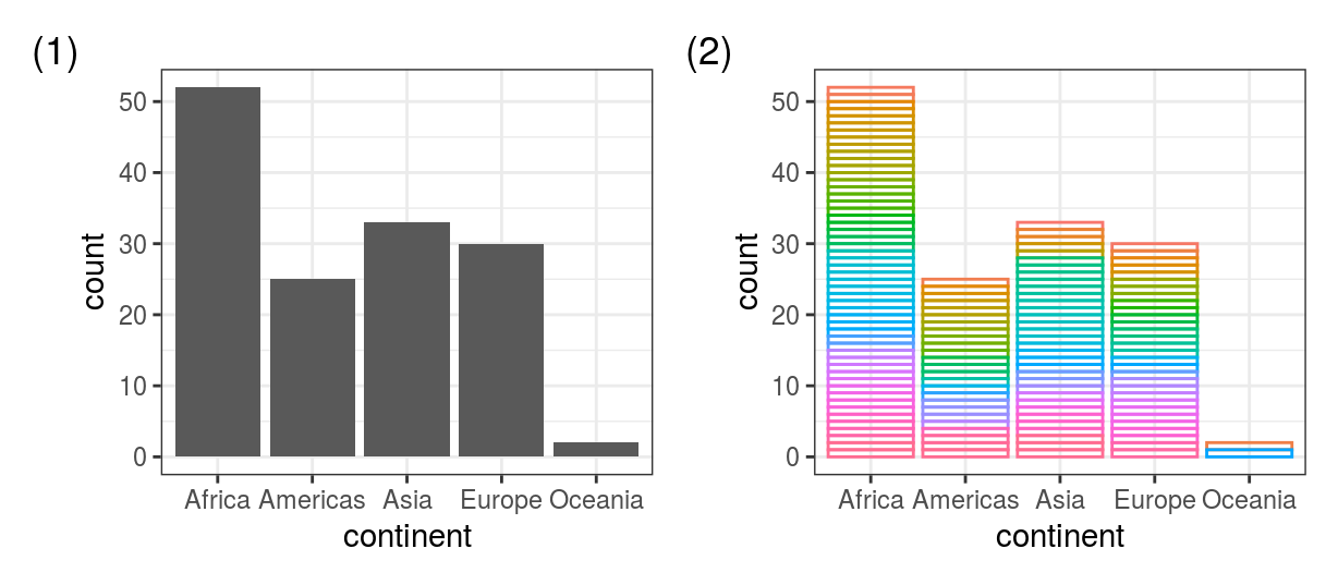
FIGURE 4.11: geom_bar() counts up the number of observations for each group. (1) gapdata2007 %>% ggplot(aes(x = continent)) + geom_bar(), (2) same + a little bit of magic to reveal the underlying data.
The first barplot in Figure 4.11 is produced with just this:
Whereas on the second one, we’ve asked geom_bar() to reveal the components (countries) in a colourful way:
gapdata2007 %>%
  ggplot(aes(x = continent, colour = country)) +
  geom_bar(fill = NA) +
  theme(legend.position = "none")
We have added theme(legend.position = "none") to remove the legend - it includes all 142 countries and is not very informative in this case.
We’re only including the colours for a bit of fun.
We’re also removing the fill by setting it to NA (fill = NA).
Note how we defined colour = country inside the aes() (as it’s a variable), but we put the fill inside geom_bar() as a constant.
This was explained in more detail in steps (3) and (4) in the ggplot anatomy Section (4.2).
4.6.3 colour vs fill
Figure 4.11 also reveals the difference between a colour and a fill.
Colour is the border around a geom, whereas fill is inside it.
Both can either be set based on a variable in your dataset (this means colour = or fill = needs to be inside the aes() function), or they could be set to a fixed colour.
R has an amazing knowledge of colour.
In addition to knowing what is “white”, “yellow”, “red”, “green” etc. (meaning we can simply do geom_bar(fill = "green")), it also knows what “aquamarine”, “blanchedalmond”, “coral”, “deeppink”, “lavender”, “deepskyblue” look like (amongst many many others; search the internet for “R colours” for a full list).
We can also use Hex colour codes, for example, geom_bar(fill = "#FF0099") is a very pretty pink.
Every single colour in the world can be represented with a Hex code, and the codes are universally known by most plotting or image making programmes.
Therefore, you can find Hex colour codes from a lot of places on the internet, or https://www.color-hex.com just to name one.
4.6.4 Proportions
Whether using geom_bar() or geom_col(), we can use fill to display proportions within bars.
Furthermore, sometimes it’s useful to set the x value to a constant - to get everything plotted together rather than separated by a variable.
So we are using aes(x = "Global", fill = continent).
Note that “Global” could be any word - since it’s quoted ggplot() won’t go looking for it in the dataset (Figure 4.12):
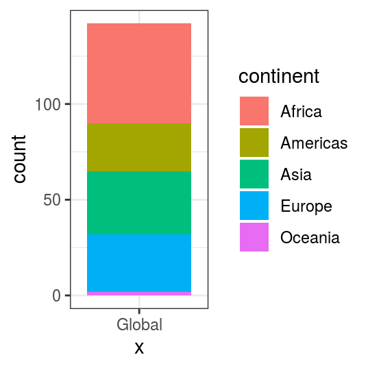
FIGURE 4.12: Number of countries in the gapminder datatset with proportions using the fill = continent aesthetic.
There are more examples of bar plots in Chapter 8.
4.6.5 Exercise
Create Figure 4.13 of life expectancies in European countries (year 2007).
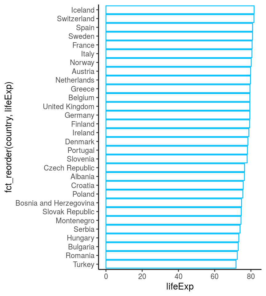
FIGURE 4.13: Barplot exercise. Life expectancies in European countries in year 2007 from the gapminder dataset.
Hints:
- If
geom_bar()doesn’t work trygeom_col()or vice versa. coord_flip()to make the bars horizontal (it flips thexandyaxes).x = countrygets the country bars plotted in alphabetical order, usex = fct_reorder(country, lifeExp)still inside theaes()to order the bars by theirlifeExpvalues. Or try one of the other variables (pop,gdpPercap) as the second argument tofct_reorder().- when using
fill = NA, you also need to include a colour; we’re usingcolour = "deepskyblue"inside thegeom_col().
The number of countries in this dataset is 142, whereas the United Nations have 193 member states.↩︎