6.9 Non-parametric tests

What if your data is a different shape to normal, or the ANOVA assumptions are not fulfilled (see linear regression chapter)? As always, be sensible and think what drives your measurements in the first place. Would your data be expected to be normally distributed given the data-generating process?

For instance, if you are examining length of hospital stay it is likely that your data are highly right skewed - most patients are discharged from hospital in a few days while a smaller number stay for a long time. Is a comparison of means ever going to be the correct approach here? Perhaps you should consider a time-to-event analysis for instance (see Chapter 10).

If a comparison of means approach is reasonable, but the normality assumption is not fulfilled there are two approaches,

Transform the data;
Perform non-parametric tests.

6.9.1 Transforming data

Remember, the Welch t-test is reasonably robust to divergence from the normality assumption, so small deviations can be safely ignored.

Otherwise, the data can be transformed to another scale to deal with a skew. A natural log scale is common.

TABLE 6.4: Transformations that can be applied to skewed data. For left skewed data, subtract all values from a constant greater than the maximum value.
Distribution	Transformation	Function
Moderate right skew (+)	Square-root	sqrt()
Substantial right skew (++)	Natural log*	log()
Substantial right skew (+++)	Base-10 log*	log10()
Note:
If data contain zero values, add a small constant to all values.

africa2002 <- gapdata %>%              # save as africa2002
  filter(year == 2002) %>%             # only 2002
  filter(continent == "Africa") %>%    # only Africa
  select(country, lifeExp) %>%         # only these variables
  mutate(
    lifeExp_log = log(lifeExp)         # log life expectancy
  )
head(africa2002)                       # inspect

## # A tibble: 6 x 3
##   country      lifeExp lifeExp_log
##   <fct>          <dbl>       <dbl>
## 1 Algeria         71.0        4.26
## 2 Angola          41.0        3.71
## 3 Benin           54.4        4.00
## 4 Botswana        46.6        3.84
## 5 Burkina Faso    50.6        3.92
## 6 Burundi         47.4        3.86

africa2002 %>% 
  # pivot lifeExp and lifeExp_log values to same column (for easy plotting):
  pivot_longer(contains("lifeExp")) %>% 
  ggplot(aes(x = value)) +             
  geom_histogram(bins = 15) +          # make histogram
  facet_wrap(~name, scales = "free")    # facet with axes free to vary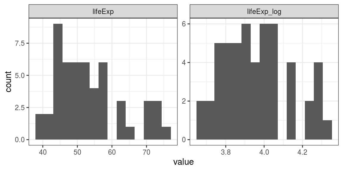

FIGURE 6.9: Histogram: Log transformation of life expectancy for countries in Africa 2002.

This has worked well here. The right skew on the Africa data has been dealt with by the transformation. A parametric test such as a t-test can now be performed.

6.9.2 Non-parametric test for comparing two groups

The Mann-Whitney U test is also called the Wilcoxon rank-sum test and uses a rank-based method to compare two groups (note the Wilcoxon signed-rank test is for paired data). Rank-based just means ordering your grouped continuous data from smallest to largest value and assigning a rank (1, 2, 3 …) to each measurement.

We can use it to test for a difference in life expectancies for African countries between 1982 and 2007. Let’s do a histogram, Q-Q plot and boxplot first.

africa_data <- gapdata %>%                          
  filter(year %in% c(1982, 2007)) %>%      # only 1982 and 2007
  filter(continent %in% c("Africa"))       # only Africa

p1 <- africa_data %>%                      # save plot as p1
  ggplot(aes(x = lifeExp)) + 
  geom_histogram(bins = 15) +
  facet_wrap(~year)

p2 <- africa_data %>%                      # save plot as p2
  ggplot(aes(sample = lifeExp)) +          # `sample` for Q-Q plot
  geom_qq() + 
  geom_qq_line(colour = "blue") + 
  facet_wrap(~year)

p3 <- africa_data %>%                      # save plot as p3
  ggplot(aes(x = factor(year),             # try without factor(year) to
             y = lifeExp)) +               # see the difference
  geom_boxplot(aes(fill = factor(year))) + # colour boxplot
  geom_jitter(alpha = 0.4) +               # add data points
  theme(legend.position = "none")          # remove legend

library(patchwork)                         # great for combining plots
p1 / p2 | p3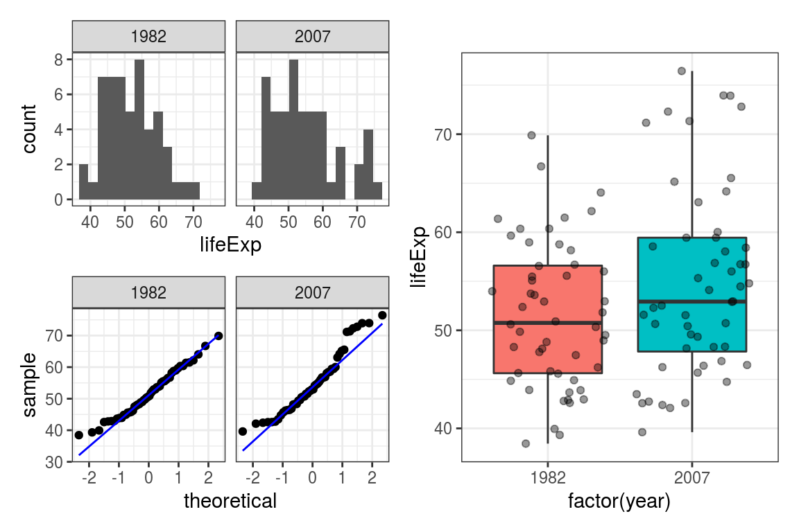

FIGURE 6.10: Panels plots: Histogram, Q-Q, boxplot for life expectancy in Africa 1992 v 2007.

The data is a little skewed based on the histograms and Q-Q plots. The difference between 1982 and 2007 is not particularly striking on the boxplot.

africa_data %>% 
  wilcox.test(lifeExp ~ year, data = .)

## 
##  Wilcoxon rank sum test with continuity correction
## 
## data:  lifeExp by year
## W = 1130, p-value = 0.1499
## alternative hypothesis: true location shift is not equal to 0

6.9.3 Non-parametric test for comparing more than two groups

The non-parametric equivalent to ANOVA, is the Kruskal-Wallis test. It can be used in base R, or via the finalfit package below.

library(broom)
gapdata %>% 
  filter(year == 2007) %>% 
  filter(continent %in% c("Americas", "Europe", "Asia")) %>% 
  kruskal.test(lifeExp~continent, data = .) %>% 
  tidy()

## # A tibble: 1 x 4
##   statistic   p.value parameter method                      
##       <dbl>     <dbl>     <int> <chr>                       
## 1      21.6 0.0000202         2 Kruskal-Wallis rank sum test