11.8 Handling missing data: MAR

But life is rarely that simple.

Considering that the smoking variable is more likely to be missing if the patient is female (missing_compare shows a relationship). But, say, that the missing values are not different from the observed values. Missingness is then MAR.

If we simply drop all the patients for whom smoking is missing (list-wise deletion), then we drop relatively more females than men. This may have consequences for our conclusions if sex is associated with our explanatory variable of interest or outcome.

11.8.1 Common solution: Multivariate Imputation by Chained Equations (mice)

mice is our go to package for multiple imputation. That’s the process of filling in missing data using a best-estimate from all the other data that exists. When first encountered, this may not sound like a good idea.

However, taking our simple example, if missingness in smoking is predicted strongly by sex (and other observed variables), and the values of the missing data are random, then we can impute (best-guess) the missing smoking values using sex and other variables in the dataset.

Imputation is not usually appropriate for the explanatory variable of interest or the outcome variable, although these can be used to impute other variables. In both cases, the hypothesis is that there is a meaningful association with other variables in the dataset, therefore it doesn’t make sense to use these variables to impute them.

The process of multiple imputation involves:

• Impute missing data m times, which results in m complete datasets
• Diagnose the quality of the imputed values
• Analyse each completed dataset
• Pool the results of the repeated analyses

We will present a mice() example here. The package is well documented, and there are a number of checks and considerations that should be made to inform the imputation process. Read the documentation carefully prior to doing this yourself.

Note also missing_predictorMatrix() from finalfit. This provides a straightforward way to include or exclude variables to be imputed or to be used for imputation.

Impute

# Multivariate Imputation by Chained Equations (mice)
library(finalfit)
library(dplyr)
library(mice)
explanatory <- c("age", "sex.factor", 
                 "nodes", "obstruct.factor", "smoking_mar")
dependent <- "mort_5yr"

Choose which variable to input missing values for and which variables to use for the imputation process.

colon_s %>% 
  select(dependent, explanatory) %>% 
  missing_predictorMatrix(
    drop_from_imputed = c("obstruct.factor", "mort_5yr")
  ) -> predM

Make 10 imputed datasets and run our logistic regression analysis on each set.

fits <- colon_s %>% 
  select(dependent, explanatory) %>% 
  
  # Usually run imputation with 10 imputed sets, 4 here for demonstration
  mice(m = 4, predictorMatrix = predM) %>% 
  
  # Run logistic regression on each imputed set
  with(glm(formula(ff_formula(dependent, explanatory)), 
           family="binomial"))

## 
##  iter imp variable
##   1   1  mort_5yr  nodes  obstruct.factor  smoking_mar
##   1   2  mort_5yr  nodes  obstruct.factor  smoking_mar
##   1   3  mort_5yr  nodes  obstruct.factor  smoking_mar
##   1   4  mort_5yr  nodes  obstruct.factor  smoking_mar
##   2   1  mort_5yr  nodes  obstruct.factor  smoking_mar
##   2   2  mort_5yr  nodes  obstruct.factor  smoking_mar
##   2   3  mort_5yr  nodes  obstruct.factor  smoking_mar
##   2   4  mort_5yr  nodes  obstruct.factor  smoking_mar
##   3   1  mort_5yr  nodes  obstruct.factor  smoking_mar
##   3   2  mort_5yr  nodes  obstruct.factor  smoking_mar
##   3   3  mort_5yr  nodes  obstruct.factor  smoking_mar
##   3   4  mort_5yr  nodes  obstruct.factor  smoking_mar
##   4   1  mort_5yr  nodes  obstruct.factor  smoking_mar
##   4   2  mort_5yr  nodes  obstruct.factor  smoking_mar
##   4   3  mort_5yr  nodes  obstruct.factor  smoking_mar
##   4   4  mort_5yr  nodes  obstruct.factor  smoking_mar
##   5   1  mort_5yr  nodes  obstruct.factor  smoking_mar
##   5   2  mort_5yr  nodes  obstruct.factor  smoking_mar
##   5   3  mort_5yr  nodes  obstruct.factor  smoking_mar
##   5   4  mort_5yr  nodes  obstruct.factor  smoking_mar

Extract metrics from each model

# Examples of extracting metrics from fits and taking the mean
## AICs
fits %>% 
  getfit() %>% 
  purrr::map(AIC) %>%
  unlist() %>% 
  mean()

## [1] 1193.679

# C-statistic
fits %>% 
  getfit() %>% 
  purrr::map(~ pROC::roc(.x$y, .x$fitted)$auc) %>% 
  unlist() %>% 
  mean()

## [1] 0.6789003

Pool models together

# Pool  results
fits_pool <- fits %>% 
  pool()

## Can be passed to or_plot
colon_s %>% 
  or_plot(dependent, explanatory, glmfit = fits_pool, table_text_size=4)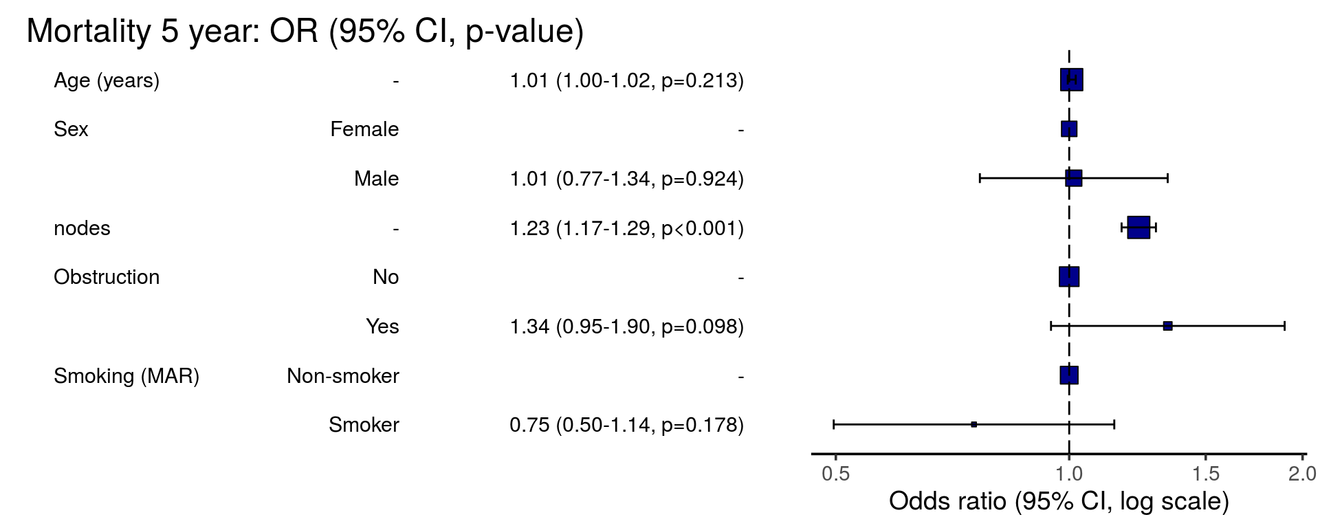

# Summarise and put in table
fit_imputed <- fits_pool %>%                                  
  fit2df(estimate_name = "OR (multiple imputation)", exp = TRUE)

# Use finalfit merge methods to create and compare results
explanatory <- c("age", "sex.factor", 
                 "nodes", "obstruct.factor", "smoking_mar")

table_uni_multi <- colon_s %>% 
  finalfit(dependent, explanatory, keep_fit_id = TRUE) 

explanatory = c("age", "sex.factor", 
                "nodes", "obstruct.factor")

fit_multi_no_smoking <- colon_s %>% 
  glmmulti(dependent, explanatory) %>% 
  fit2df(estimate_suffix = " (multivariable without smoking)") 

# Combine to final table
table_imputed <- 
  table_uni_multi %>% 
  ff_merge(fit_multi_no_smoking) %>% 
  ff_merge(fit_imputed, last_merge = TRUE)

TABLE 7.1: Regression analysis with missing data: Multiple imputation using mice().

Dependent: Mortality 5 year		Alive	Died	OR (univariable)	OR (multivariable)	OR (multivariable without smoking)	OR (multiple imputation)
Age (years)	Mean (SD)	59.8 (11.4)	59.9 (12.5)	1.00 (0.99-1.01, p=0.986)	1.02 (1.01-1.04, p=0.004)	1.01 (1.00-1.02, p=0.122)	1.01 (1.00-1.02, p=0.213)
Sex	Female	243 (55.6)	194 (44.4)
	Male	268 (56.1)	210 (43.9)	0.98 (0.76-1.27, p=0.889)	0.97 (0.69-1.34, p=0.836)	0.98 (0.74-1.30, p=0.890)	1.01 (0.77-1.34, p=0.924)
nodes	Mean (SD)	2.7 (2.4)	4.9 (4.4)	1.24 (1.18-1.30, p<0.001)	1.28 (1.21-1.37, p<0.001)	1.25 (1.19-1.32, p<0.001)	1.23 (1.17-1.29, p<0.001)
Obstruction	No	408 (56.7)	312 (43.3)
	Yes	89 (51.1)	85 (48.9)	1.25 (0.90-1.74, p=0.189)	1.49 (1.00-2.22, p=0.052)	1.36 (0.95-1.93, p=0.089)	1.34 (0.95-1.90, p=0.098)
Smoking (MAR)	Non-smoker	312 (54.0)	266 (46.0)
	Smoker	87 (62.6)	52 (37.4)	0.70 (0.48-1.02, p=0.067)	0.77 (0.51-1.16, p=0.221)		0.75 (0.50-1.14, p=0.178)

By examining the coefficients, the effect of the imputation compared with the complete case analysis can be seen.

Other considerations

• Omit the variable
• Model the missing data

As above, if the variable does not appear to be important, it may be omitted from the analysis. A sensitivity analysis in this context is another form of imputation. But rather than using all other available information to best-guess the missing data, we simply assign the value as above. Imputation is therefore likely to be more appropriate.

There is an alternative method to model the missing data for the categorical in this setting – just consider the missing data as a factor level. This has the advantage of simplicity, with the disadvantage of increasing the number of terms in the model.

library(dplyr)
explanatory = c("age", "sex.factor", 
                "nodes", "obstruct.factor", "smoking_mar")
fit_explicit_na = colon_s %>% 
  mutate(
    smoking_mar = forcats::fct_explicit_na(smoking_mar)
  ) %>% 
  finalfit(dependent, explanatory)

TABLE 9.5: Regression analysis with missing data: Explicitly modelling missing data.

Dependent: Mortality 5 year		Alive	Died	OR (univariable)	OR (multivariable)
Age (years)	Mean (SD)	59.8 (11.4)	59.9 (12.5)	1.00 (0.99-1.01, p=0.986)	1.01 (1.00-1.02, p=0.114)
Sex	Female	243 (55.6)	194 (44.4)
	Male	268 (56.1)	210 (43.9)	0.98 (0.76-1.27, p=0.889)	0.95 (0.71-1.28, p=0.743)
nodes	Mean (SD)	2.7 (2.4)	4.9 (4.4)	1.24 (1.18-1.30, p<0.001)	1.25 (1.19-1.32, p<0.001)
Obstruction	No	408 (56.7)	312 (43.3)
	Yes	89 (51.1)	85 (48.9)	1.25 (0.90-1.74, p=0.189)	1.35 (0.95-1.92, p=0.099)
Smoking (MAR)	Non-smoker	312 (54.0)	266 (46.0)
	Smoker	87 (62.6)	52 (37.4)	0.70 (0.48-1.02, p=0.067)	0.78 (0.52-1.17, p=0.233)
	(Missing)	112 (56.6)	86 (43.4)	0.90 (0.65-1.25, p=0.528)	0.85 (0.59-1.23, p=0.390)