9.3 Data preparation and exploratory analysis

9.3.1 The Question (2)

We will go on to explore the boot::melanoma dataset introduced in Chapter 8. The data consist of measurements made on patients after surgery to remove the melanoma skin cancer in the University Hospital of Odense, Denmark, between 1962 and 1977.

Malignant melanoma is an aggressive and highly invasive cancer, making it difficult to treat.

To determine how advanced it is, staging is based on the depth of the tumour. The current TNM classification cut-offs are:

T1: \(\leq\) 1.0 mm depth
T2: 1.1 to 2.0 mm depth
T3: 2.1 to 4.0 mm depth
T4: > 4.0 mm depth

This will be important in our analysis as we will create a new variable based upon this.

Using logistic regression, we will investigate factors associated with death from malignant melanoma with particular interest in tumour ulceration.

9.3.2 Get the data

The Help page (F1 on boot::melanoma) gives us its data dictionary including the definition of each variable and the coding used.

melanoma <- boot::melanoma

9.3.3 Check the data

As before, always carefully check and clean new dataset before you start the analysis.

library(tidyverse)
library(finalfit)
melanoma %>% glimpse()
melanoma %>% ff_glimpse()

9.3.4 Recode the data

We have seen some of this already (Section 8.5: Recode data), but for this particular analysis we will recode some further variables.

library(tidyverse)
library(finalfit)
melanoma <- melanoma %>% 
  mutate(sex.factor = factor(sex) %>%          
           fct_recode("Female" = "0",
                      "Male"   = "1") %>% 
           ff_label("Sex"),   
         
         ulcer.factor = factor(ulcer) %>% 
           fct_recode("Present" = "1",
                      "Absent"  = "0") %>% 
           ff_label("Ulcerated tumour"),
         
         age  = ff_label(age,  "Age (years)"),
         year = ff_label(year, "Year"),
         
         status.factor = factor(status) %>% 
           fct_recode("Died melanoma"  = "1",
                      "Alive" = "2",
                      "Died - other" = "3") %>% 
           fct_relevel("Alive") %>% 
           ff_label("Status"),
         
         t_stage.factor = 
           thickness %>% 
           cut(breaks = c(0, 1.0, 2.0, 4.0, 
                          max(thickness, na.rm=TRUE)),
               include.lowest = TRUE)
  )

Check the cut() function has worked:

melanoma$t_stage.factor %>% levels()

## [1] "[0,1]"    "(1,2]"    "(2,4]"    "(4,17.4]"

Recode for ease.

melanoma <- melanoma %>% 
  mutate(
    t_stage.factor = 
      fct_recode(t_stage.factor,
                 "T1" = "[0,1]",
                 "T2" = "(1,2]",
                 "T3" = "(2,4]",
                 "T4" = "(4,17.4]") %>% 
      ff_label("T-stage")
  )

We will now consider our outcome variable. With a binary outcome and health data, we often have to make a decision as to when to determine if that variable has occurred or not. In the next chapter we will look at survival analysis where this requirement is not needed.

Our outcome of interest is death from melanoma, but we need to decide when to define this.

A quick histogram of time stratified by status.factor helps. We can see that most people who died from melanoma did so before 5 years (Figure 9.7). We can also see that the status most of those who did not die is known beyond 5 years.

library(ggplot2)
melanoma %>% 
  ggplot(aes(x = time/365)) + 
  geom_histogram() + 
  facet_grid(. ~ status.factor)

## `stat_bin()` using `bins = 30`. Pick better value with `binwidth`.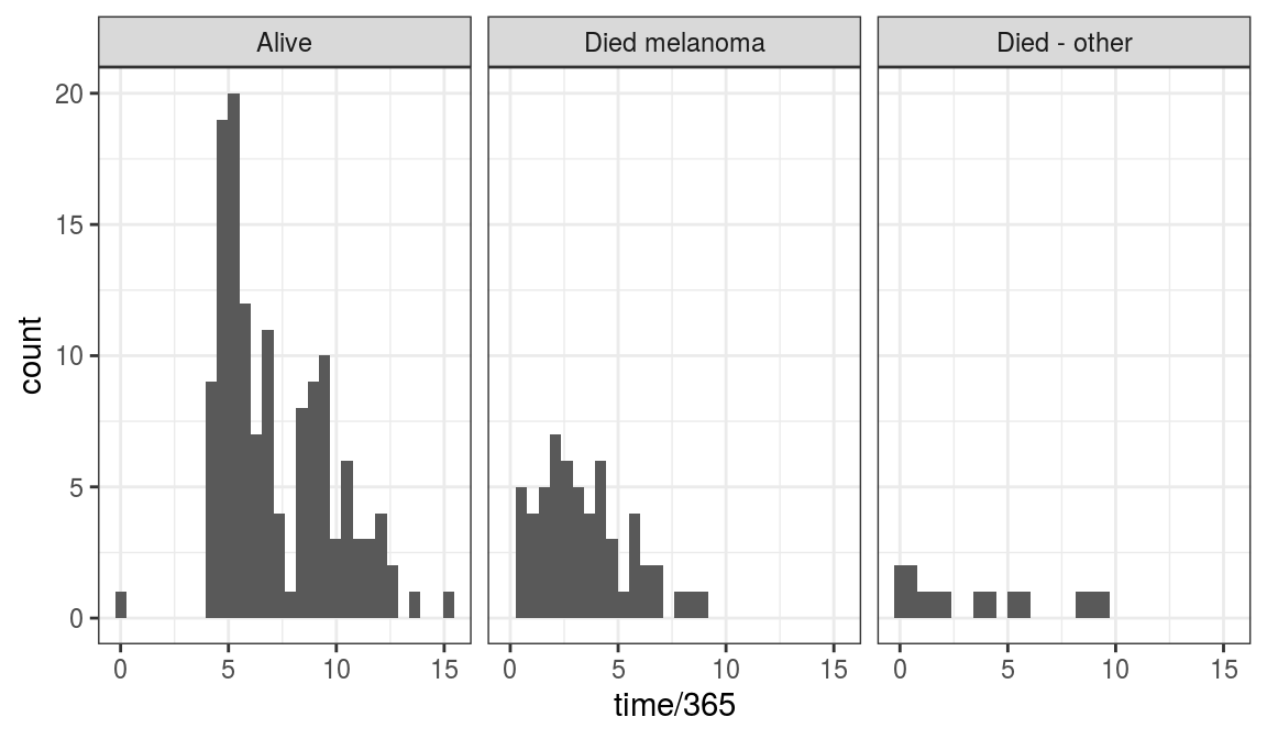

FIGURE 9.7: Time to outcome/follow-up times for patients in the melanoma dataset.

Let’s decide then to look at 5-year mortality from melanoma. The definition of this will be at 5 years after surgery, who had died from melanoma and who had not.

# 5-year mortality
melanoma <- melanoma %>% 
  mutate(
    mort_5yr = 
      if_else((time/365) < 5 & 
                (status == 1), 
              "Yes",          # then
              "No") %>%       # else
      fct_relevel("No") %>% 
      ff_label("5-year survival")
  )

9.3.5 Plot the data

We are interested in the association between tumour ulceration and outcome (Figure 9.8).

p1 <- melanoma %>% 
  ggplot(aes(x = ulcer.factor, fill = mort_5yr)) + 
  geom_bar() + 
  theme(legend.position = "none")

p2 <- melanoma %>% 
  ggplot(aes(x = ulcer.factor, fill = mort_5yr)) + 
  geom_bar(position = "fill") + 
  ylab("proportion")

library(patchwork)
p1 + p2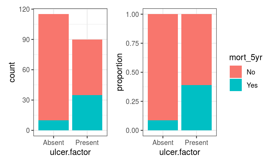

FIGURE 9.8: Exploration ulceration and outcome (5-year mortality).

As we might have anticipated from our work in the previous chapter, 5-year mortality is higher in patients with ulcerated tumours compared with those with non-ulcerated tumours.

We are also interested in other variables that may be associated with tumour ulceration. If they are also associated with our outcome, then they will confound the estimate of the direct effect of tumour ulceration.

We can plot out these relationships, or tabulate them instead.

9.3.6 Tabulate data

We will use the convenient summary_factorlist() function from the finalfit package to look for differences across other variables by tumour ulceration.

library(finalfit)
dependent <- "ulcer.factor"
explanatory <- c("age", "sex.factor", "year", "t_stage.factor")
melanoma %>% 
  summary_factorlist(dependent, explanatory, p = TRUE,
                     add_dependent_label = TRUE)

TABLE 9.1: Multiple variables by explanatory variable of interest: Malignant melanoma ulceration by patient and disease variables.
Dependent: Ulcerated tumour		Absent	Present	p
Age (years)	Mean (SD)	50.6 (15.9)	54.8 (17.4)	0.072
Sex	Female	79 (68.7)	47 (52.2)	0.024
	Male	36 (31.3)	43 (47.8)
Year	Mean (SD)	1970.0 (2.7)	1969.8 (2.4)	0.637
T-stage	T1	51 (44.3)	5 (5.6)	<0.001
	T2	36 (31.3)	17 (18.9)
	T3	21 (18.3)	30 (33.3)
	T4	7 (6.1)	38 (42.2)

It appears that patients with ulcerated tumours were older, more likely to be male, and had thicker/higher stage tumours. It is important therefore to consider inclusion of these variables in a regression model.