12.6 Interface and outputting

12.6.1 Running code and chunks, knitting

Figure 12.4 shows the various controls for running chunks and producing an output document. Code can be run line-by-line using Ctrl+Enter as you are used to. There are options for running all the chunks above the current chunk you are working on. This is useful as a chunk you are working on will often rely on objects created in preceding chunks.

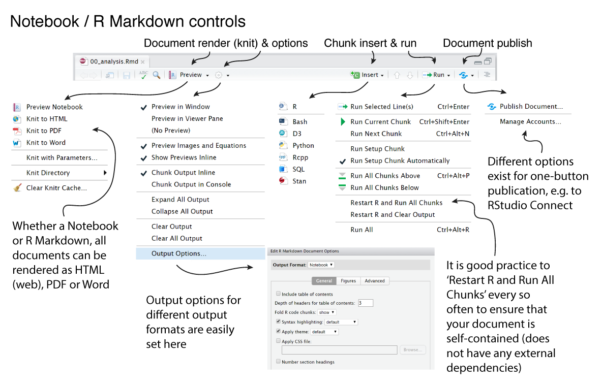
FIGURE 12.4: Chunk and document options in Notebook/Markdown files.

It is good practice to use the Restart R and Run All Chunks option in the Run menu every so often. This ensures that all the code in your document is self-contained and is not relying on an object in the environment which you have created elsewhere. If this was the case, it will fail when rendering a Markdown document.

Probably the most important engine behind the RStudio Notebooks functionality is the knitr package by Yihui Xie.

Not knitting like your granny does, but rendering a Markdown document into an output file, such as HTML, PDF or Word. There are many options which can be applied in order to achieve the desired output. Some of these have been specifically coded into RStudio (Figure 12.4).

PDF document creation requires a LaTeX distribution to be installed on your computer. Depending on what system you are using, this may be setup already. An easy way to do this is using the tinytex package.

```{r}
install.packages("tinytex")
# Restart R, then run
tinytex::install_tinytex()
```

In the next chapter we will focus on the details of producing a polished final document.