7.2 Fitting simple models
7.2.1 The Question (2)
We are interested in modelling the change in life expectancy for different countries over the past 60 years.
7.2.2 Get the data
7.2.3 Check the data
Always check a new dataset, as described in Section 6.3.
7.2.4 Plot the data
Let’s plot the life expectancies in European countries over the past 60 years, focussing on the UK and Turkey.
We can add in simple best fit lines using geom_smooth().
gapdata %>%
  filter(continent == "Europe") %>%    # Europe only
  ggplot(aes(x = year, y = lifeExp)) + # lifeExp~year
  geom_point() +                       # plot points
  facet_wrap(~ country) +              # facet by country
  scale_x_continuous(
    breaks = c(1960, 2000)) +          # adjust x-axis
  geom_smooth(method = "lm")           # add regression lines
## `geom_smooth()` using formula 'y ~ x'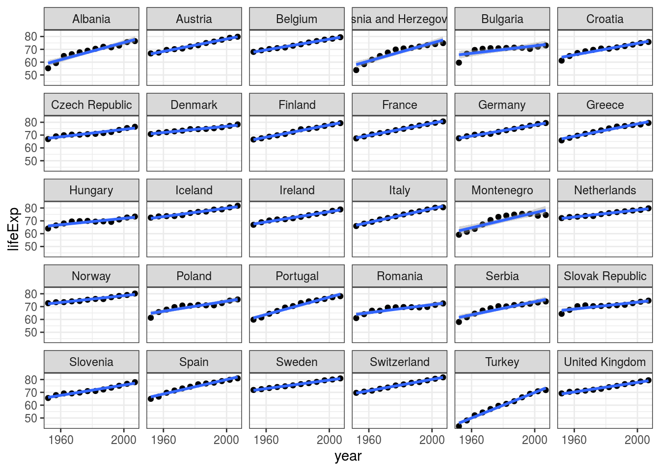
FIGURE 7.8: Scatter plots with linear regression lines: Life expectancy by year in European countries.
7.2.5 Simple linear regression
As you can see, ggplot() is very happy to run and plot linear regression models for us.
While this is convenient for a quick look, we usually want to build, run, and explore these models ourselves.
We can then investigate the intercepts and the slope coefficients (linear increase per year):
First let’s plot two countries to compare, Turkey and United Kingdom:
gapdata %>%
  filter(country %in% c("Turkey", "United Kingdom")) %>%
  ggplot(aes(x = year, y = lifeExp, colour = country)) +
  geom_point()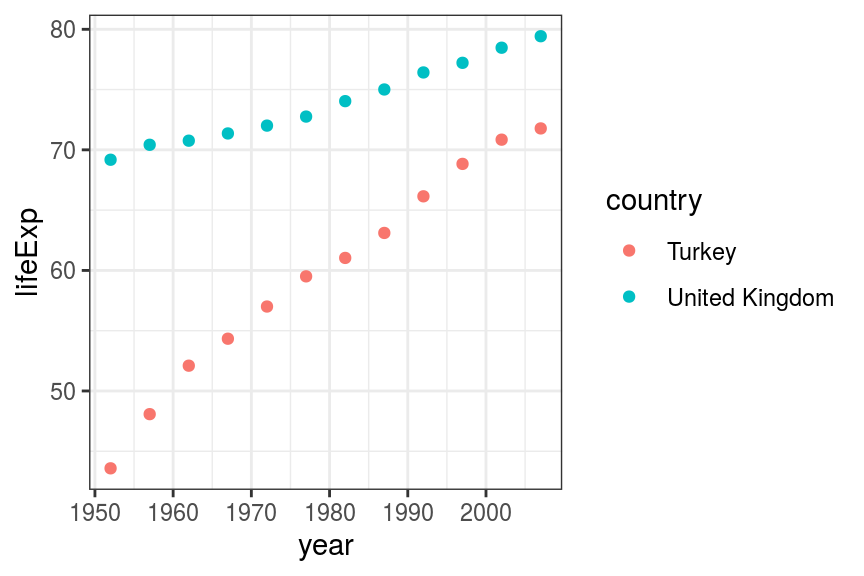
FIGURE 7.9: Scatter plot: Life expectancy by year: Turkey and United Kingdom
The two non-parallel lines may make you think of what has been discussed above (Figure 7.6).
First, let’s model the two countries separately.
# United Kingdom
fit_uk <- gapdata %>%
  filter(country == "United Kingdom") %>%
  lm(lifeExp~year, data = .)

fit_uk %>%
  summary()
##
## Call:
## lm(formula = lifeExp ~ year, data = .)
##
## Residuals:
## Min 1Q Median 3Q Max
## -0.69767 -0.31962 0.06642 0.36601 0.68165
##
## Coefficients:
## Estimate Std. Error t value Pr(>|t|)
## (Intercept) -2.942e+02 1.464e+01 -20.10 2.05e-09 ***
## year 1.860e-01 7.394e-03 25.15 2.26e-10 ***
## ---
## Signif. codes: 0 '***' 0.001 '**' 0.01 '*' 0.05 '.' 0.1 ' ' 1
##
## Residual standard error: 0.4421 on 10 degrees of freedom
## Multiple R-squared: 0.9844, Adjusted R-squared: 0.9829
## F-statistic: 632.5 on 1 and 10 DF, p-value: 2.262e-10# Turkey
fit_turkey <- gapdata %>%
filter(country == "Turkey") %>%
lm(lifeExp~year, data = .)
fit_turkey %>%
summary()##
## Call:
## lm(formula = lifeExp ~ year, data = .)
##
## Residuals:
## Min 1Q Median 3Q Max
## -2.4373 -0.3457 0.1653 0.9008 1.1033
##
## Coefficients:
## Estimate Std. Error t value Pr(>|t|)
## (Intercept) -924.58989 37.97715 -24.35 3.12e-10 ***
## year 0.49724 0.01918 25.92 1.68e-10 ***
## ---
## Signif. codes: 0 '***' 0.001 '**' 0.01 '*' 0.05 '.' 0.1 ' ' 1
##
## Residual standard error: 1.147 on 10 degrees of freedom
## Multiple R-squared: 0.9853, Adjusted R-squared: 0.9839
## F-statistic: 671.8 on 1 and 10 DF, p-value: 1.681e-10Accessing the coefficients of linear regression
A simple linear regression model will return two coefficients - the intercept and the slope (the second returned value).
Compare these coefficients to the summary() output above to see where these numbers came from.
##  (Intercept)         year
## -294.1965876 0.1859657## (Intercept) year
## -924.5898865 0.4972399The slopes make sense - the results of the linear regression say that in the UK, life expectancy increases by 0.186 every year, whereas in Turkey the change is 0.497 per year. The reason the intercepts are negative, however, may be less obvious.
In this example, the intercept is telling us that life expectancy at year 0 in the United Kingdom (some 2000 years ago) was -294 years. While this is mathematically correct (based on the data we have), it obviously makes no sense in practice. It is important to think about the range over which you can extend your model predictions, and where they just become unrealistic.
To make the intercepts meaningful, we will add in a new column called year_from1952 and re-run fit_uk and fit_turkey using year_from1952 instead of year.
gapdata <- gapdata %>%
  mutate(year_from1952 = year - 1952)

fit_uk <- gapdata %>%
  filter(country == "United Kingdom") %>%
  lm(lifeExp ~ year_from1952, data = .)

fit_turkey <- gapdata %>%
  filter(country == "Turkey") %>%
lm(lifeExp ~ year_from1952, data = .)## (Intercept) year_from1952
## 68.8085256 0.1859657## (Intercept) year_from1952
## 46.0223205 0.4972399Now, the updated results tell us that in year 1952, the life expectancy in the United Kingdom was 69 years. Note that the slopes do not change. There was nothing wrong with the original model and the results were correct, the intercept was just not meaningful.
Accessing all model information tidy() and glance()
In the fit_uk and fit_turkey examples above, we were using fit_uk %>% summary() to get R to print out a summary of the model.
This summary is not, however, in a rectangular shape so we can’t easily access the values or put them in a table/use as information on plot labels.
We use the tidy() function from library(broom) to get the variable(s) and specific values in a nice tibble:
## # A tibble: 2 x 5
##   term          estimate std.error statistic  p.value
##   <chr>            <dbl>     <dbl>     <dbl>    <dbl>
## 1 (Intercept)     68.8     0.240       287.  6.58e-21
## 2 year_from1952    0.186   0.00739      25.1 2.26e-10
In the tidy() output, the column estimate includes both the intercepts and slopes.
And we use the glance() function to get overall model statistics (mostly the r.squared).
## # A tibble: 1 x 12
##   r.squared adj.r.squared sigma statistic  p.value    df logLik   AIC   BIC
##       <dbl>         <dbl> <dbl>     <dbl>    <dbl> <dbl>  <dbl> <dbl> <dbl>
## 1     0.984         0.983 0.442      633. 2.26e-10     1  -6.14  18.3  19.7
## # … with 3 more variables: deviance <dbl>, df.residual <int>, nobs <int>
7.2.6 Multivariable linear regression
Multivariable linear regression includes more than one explanatory variable. There are a few ways to include more variables, depending on whether they should share the intercept and how they interact:
Simple linear regression (exactly one predictor variable):
myfit = lm(lifeExp ~ year, data = gapdata)
Multivariable linear regression (additive):
myfit = lm(lifeExp ~ year + country, data = gapdata)
Multivariable linear regression (interaction):
myfit = lm(lifeExp ~ year * country, data = gapdata)
This equivalent to:
myfit = lm(lifeExp ~ year + country + year:country, data = gapdata)
These examples of multivariable regression include two variables: year and country, but we could include more by adding them with +, it does not just have to be two.
We will now create three different linear regression models to further illustrate the difference between a simple model, additive model, and multiplicative model.
Model 1: year only
# UK and Turkey dataset
gapdata_UK_T <- gapdata %>%
  filter(country %in% c("Turkey", "United Kingdom"))

fit_both1 <- gapdata_UK_T %>%
  lm(lifeExp ~ year_from1952, data = .)
fit_both1
##
## Call:
## lm(formula = lifeExp ~ year_from1952, data = .)
##
## Coefficients:
## (Intercept) year_from1952
## 57.4154 0.3416gapdata_UK_T %>%
mutate(pred_lifeExp = predict(fit_both1)) %>%
ggplot() +
geom_point(aes(x = year, y = lifeExp, colour = country)) +
geom_line(aes(x = year, y = pred_lifeExp))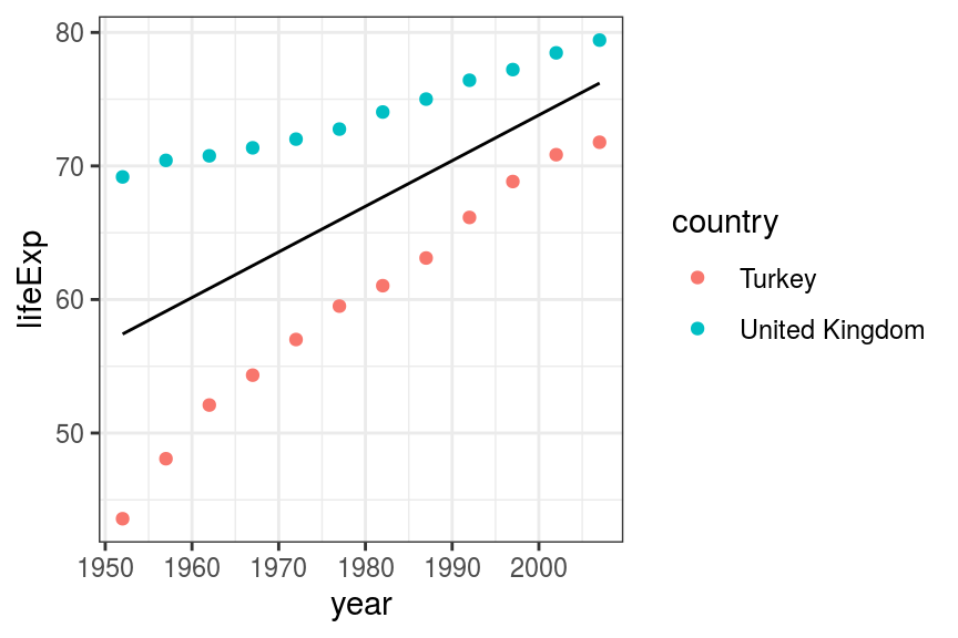
FIGURE 6.7: Scatter and line plot. Life expectancy in Turkey and the UK - univariable fit.
By fitting to year only (lifeExp ~ year_from1952), the model ignores country.
This gives us a fitted line which is the average of life expectancy in the UK and Turkey.
This may be desirable, depending on the question.
But here we want to best describe the data.
How we made the plot and what does predict() do?
Previously, we were using geom_smooth(method = "lm") to conveniently add linear regression lines on a scatter plot.
When a scatter plot includes categorical value (e.g., the points are coloured by a variable), the regression lines geom_smooth() draws are multiplicative.
That is great, and almost always exactly what we want.
Here, however, to illustrate the difference between the different models, we will have to use the predict() model and geom_line() to have full control over the plotted regression lines.
gapdata_UK_T %>%
  mutate(pred_lifeExp = predict(fit_both1)) %>%
  select(country, year, lifeExp, pred_lifeExp) %>%
  group_by(country) %>%
  slice(1, 6, 12)
## # A tibble: 6 x 4
## # Groups: country [2]
## country year lifeExp pred_lifeExp
## <fct> <int> <dbl> <dbl>
## 1 Turkey 1952 43.6 57.4
## 2 Turkey 1977 59.5 66.0
## 3 Turkey 2007 71.8 76.2
## 4 United Kingdom 1952 69.2 57.4
## 5 United Kingdom 1977 72.8 66.0
## 6 United Kingdom 2007 79.4 76.2Note how the slice() function recognises group_by() and in this case shows us the 1st, 6th, and 12th observation within each group.
Model 2: year + country
##
## Call:
## lm(formula = lifeExp ~ year_from1952 + country, data = .)
##
## Coefficients:
##           (Intercept)          year_from1952  countryUnited Kingdom
##               50.3023                 0.3416                14.2262
gapdata_UK_T %>%
mutate(pred_lifeExp = predict(fit_both2)) %>%
ggplot() +
geom_point(aes(x = year, y = lifeExp, colour = country)) +
geom_line(aes(x = year, y = pred_lifeExp, colour = country))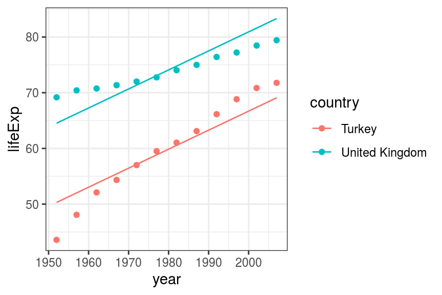
FIGURE 7.10: Scatter and line plot. Life expectancy in Turkey and the UK - multivariable additive fit.
This is better, by including country in the model, we now have fitted lines more closely representing the data. However, the lines are constrained to be parallel. This is the additive model that was discussed above. We need to include an interaction term to allow the effect of year on life expectancy to vary by country in a non-additive manner.
Model 3: year * country
##
## Call:
## lm(formula = lifeExp ~ year_from1952 * country, data = .)
##
## Coefficients:
##                         (Intercept)                        year_from1952
##                             46.0223                               0.4972
##               countryUnited Kingdom  year_from1952:countryUnited Kingdom
##                             22.7862                              -0.3113
gapdata_UK_T %>%
mutate(pred_lifeExp = predict(fit_both3)) %>%
ggplot() +
geom_point(aes(x = year, y = lifeExp, colour = country)) +
geom_line(aes(x = year, y = pred_lifeExp, colour = country))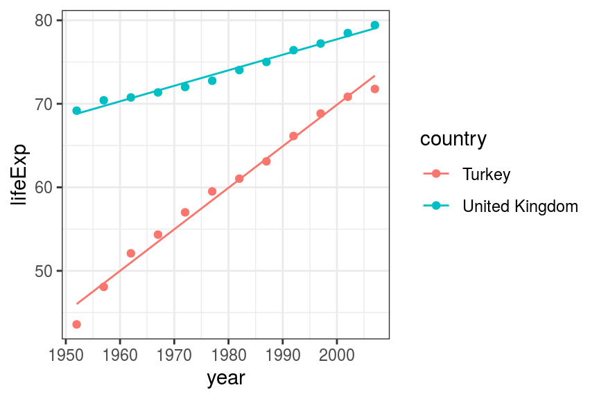
FIGURE 6.8: Scatter and line plot. Life expectancy in Turkey and the UK - multivariable multiplicative fit.
This fits the data much better than the previous two models.
You can check the R-squared using summary(fit_both3).
Advanced tip: we can apply a function on multiple objects at once by putting them in a list() and using a map_() function from the purrr package. library(purrr) gets installed and loaded with library(tidyverse), but it is outside the scope of this book. Do look it up once you get a little more comfortable with using R, and realise that you are starting to do similar things over and over again. For example, this code:
mod_stats1 <- glance(fit_both1)
mod_stats2 <- glance(fit_both2)
mod_stats3 <- glance(fit_both3)

bind_rows(mod_stats1, mod_stats2, mod_stats3)
returns the exact same thing as:
## # A tibble: 3 x 12
##   r.squared adj.r.squared sigma statistic  p.value    df logLik   AIC   BIC
##       <dbl>         <dbl> <dbl>     <dbl>    <dbl> <dbl>  <dbl> <dbl> <dbl>
## 1     0.373         0.344 7.98       13.1 1.53e- 3     1  -82.9 172.  175.
## 2     0.916         0.908 2.99      114.  5.18e-12     2  -58.8 126.  130.
## 3     0.993         0.992 0.869     980.  7.30e-22     3  -28.5  67.0  72.9
## # … with 3 more variables: deviance <dbl>, df.residual <int>, nobs <int>
What happens here is that map_df() applies a function on each object in the list it gets passed, and returns a df (data frame). In this case, the function is glance() (note that once inside map_df(), glance does not have its own brackets.
7.2.7 Check assumptions
The assumptions of linear regression can be checked with diagnostic plots, either by passing the fitted object (lm() output) to base R plot(), or by using the more convenient function below.
## Warning: `arrange_()` is deprecated as of dplyr 0.7.0.
## Please use `arrange()` instead.
## See vignette('programming') for more help
## This warning is displayed once every 8 hours.
## Call `lifecycle::last_warnings()` to see where this warning was generated.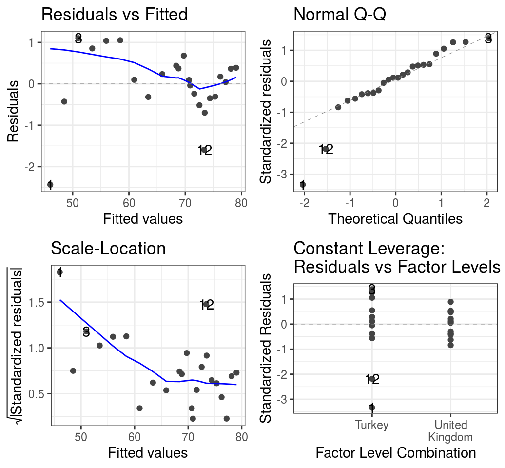
FIGURE 7.11: Diagnostic plots. Life expectancy in Turkey and the UK - multivariable multiplicative model.