4.4 Scatter plots/bubble plots

The ggplot anatomy (Section 4.2) covered both scatter and strip plots (both created with geom_point()). Another cool thing about this geom is that adding a size aesthetic makes it into a bubble plot. For example, let’s size the points by population.

As you would expect from a “grammar of graphics plot”, this is as simple as adding size = pop as an aesthetic:

gapdata2007 %>% 
  ggplot(aes(x = gdpPercap/1000, y = lifeExp, size = pop)) +
  geom_point()

With increased bubble sizes, there is some overplotting, so let’s make the points hollow (shape = 1) and slightly transparent (alpha = 0.5):

gapdata2007 %>% 
  ggplot(aes(x = gdpPercap/1000, y = lifeExp, size = pop)) +
  geom_point(shape = 1, alpha = 0.5)

The resulting bubble plots are shown in Figure 4.6.

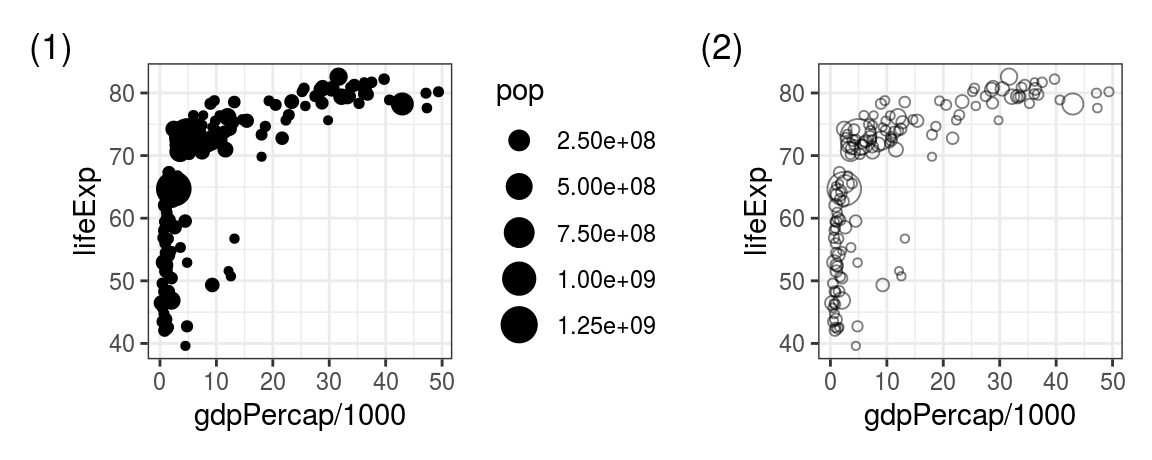
FIGURE 4.6: Turn the scatter plot from Figure 4.1:(2) to a bubble plot by (1) adding size = pop inside the aes(), (2) make the points hollow and transparent.

Alpha is an aesthetic to make geoms transparent, its values can range from 0 (invisible) to 1 (solid).