6.7 Compare the means of more than two groups

It may be that our question is set around a hypothesis involving more than two groups. For example, we may be interested in comparing life expectancy across 3 continents such as the Americas, Europe and Asia.

6.7.1 Plot the data

gapdata %>% 
  filter(year == 2007) %>% 
  filter(continent %in% 
           c("Americas", "Europe", "Asia")) %>% 
  ggplot(aes(x = continent, y=lifeExp)) +
  geom_boxplot()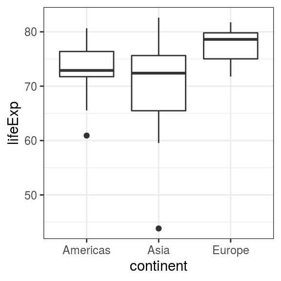

FIGURE 6.7: Boxplot: Life expectancy in selected continents for 2007.

6.7.2 ANOVA

Analysis of variance is a collection of statistical tests which can be used to test the difference in means between two or more groups.

In base R form, it produces an ANOVA table which includes an F-test. This so-called omnibus test tells you whether there are any differences in the comparison of means of the included groups. Again, it is important to plot carefully and be clear what question you are asking.

aov_data <- gapdata %>% 
  filter(year == 2007) %>% 
  filter(continent %in% c("Americas", "Europe", "Asia"))

fit = aov(lifeExp ~ continent, data = aov_data) 
summary(fit)

##             Df Sum Sq Mean Sq F value   Pr(>F)    
## continent    2  755.6   377.8   11.63 3.42e-05 ***
## Residuals   85 2760.3    32.5                     
## ---
## Signif. codes:  0 '***' 0.001 '**' 0.01 '*' 0.05 '.' 0.1 ' ' 1

We can conclude from the significant F-test that the mean life expectancy across the three continents is not the same. This does not mean that all included groups are significantly different from each other. As above, the output can be neatened up using the tidy function.

library(broom)
gapdata %>% 
  filter(year == 2007) %>% 
  filter(continent %in% c("Americas", "Europe", "Asia")) %>% 
  aov(lifeExp~continent, data = .) %>% 
  tidy()

## # A tibble: 2 x 6
##   term         df sumsq meansq statistic    p.value
##   <chr>     <dbl> <dbl>  <dbl>     <dbl>      <dbl>
## 1 continent     2  756.  378.       11.6  0.0000342
## 2 Residuals    85 2760.   32.5      NA   NA

6.7.3 Assumptions

As with the normality assumption of the t-test (for example, Sections 6.4.1 and 6.4.2), there are assumptions of the ANOVA model. These assumptions are shared with linear regression and are covered in the next chapter, as linear regression lends itself to illustrate and explain these concepts well. Suffice to say that diagnostic plots can be produced to check that the assumptions are fulfilled. library(ggfortify) includes a function called autoplot() that can be used to quickly create diagnostic plots, including the Q-Q plot that we showed before:

library(ggfortify)
autoplot(fit)

## Warning: `arrange_()` is deprecated as of dplyr 0.7.0.
## Please use `arrange()` instead.
## See vignette('programming') for more help
## This warning is displayed once every 8 hours.
## Call `lifecycle::last_warnings()` to see where this warning was generated.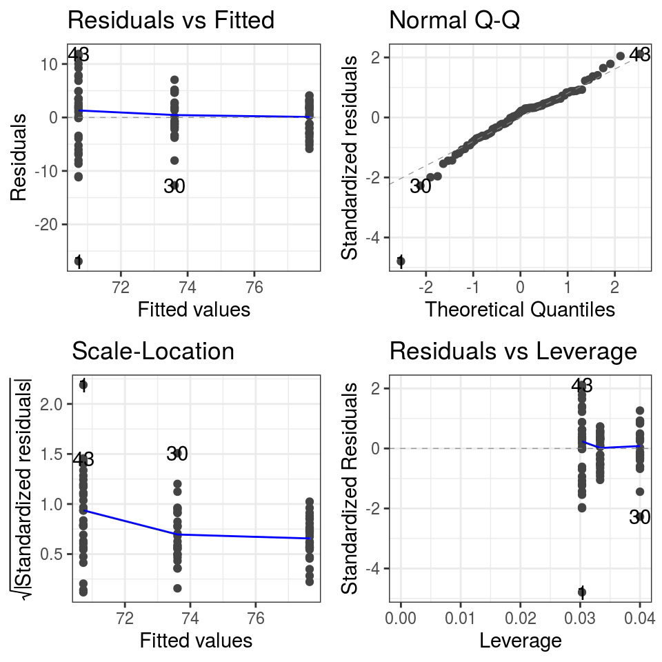

FIGURE 6.8: Diagnostic plots: ANOVA model of life expectancy by continent for 2007.