10.8 Cox proportional hazards regression
The Cox proportional hazards model is a regression model similar to those we have already dealt with. It is commonly used to investigate the association between the time to an event (such as death) and a set of explanatory variables.
Cox proportional hazards regression can be performed using survival::coxph() or the all-in-one finalfit() function.
The latter produces a table containing counts (proportions) for factors, mean (SD) for continuous variables and a univariable and multivariable CPH regression.
10.8.1 coxph()
CPH using the coxph() function produces a similar output to lm() and glm(), so it should be familiar to you now.
It can be passed to summary() as below, and also to broom::tidy() if you want to get the results into a tibble.
library(survival)
coxph(Surv(time, status_os) ~ age + sex + thickness + ulcer, data = melanoma) %>%
  summary()
## Call:
## coxph(formula = Surv(time, status_os) ~ age + sex + thickness +
## ulcer, data = melanoma)
##
## n= 205, number of events= 71
##
## coef exp(coef) se(coef) z Pr(>|z|)
## age 0.021831 1.022071 0.007752 2.816 0.004857 **
## sexMale 0.413460 1.512040 0.240132 1.722 0.085105 .
## thickness 0.099467 1.104582 0.034455 2.887 0.003891 **
## ulcerYes 0.952083 2.591100 0.267966 3.553 0.000381 ***
## ---
## Signif. codes: 0 '***' 0.001 '**' 0.01 '*' 0.05 '.' 0.1 ' ' 1
##
## exp(coef) exp(-coef) lower .95 upper .95
## age 1.022 0.9784 1.0067 1.038
## sexMale 1.512 0.6614 0.9444 2.421
## thickness 1.105 0.9053 1.0325 1.182
## ulcerYes 2.591 0.3859 1.5325 4.381
##
## Concordance= 0.739 (se = 0.03 )
## Likelihood ratio test= 47.89 on 4 df, p=1e-09
## Wald test = 46.72 on 4 df, p=2e-09
## Score (logrank) test = 52.77 on 4 df, p=1e-10The output shows the number of patients and the number of events.
The coefficient can be exponentiated and interpreted as a hazard ratio, exp(coef).
Helpfully, 95% confidence intervals are also provided.
A hazard is the term given to the rate at which events happen. The probability that an event will happen over a period of time is the hazard multiplied by the time interval. An assumption of CPH is that hazards are constant over time (see below).
For a given predictor then, the hazard in one group (say males) would be expected to be a constant proportion of the hazard in another group (say females). The ratio of these hazards is, unsurprisingly, the hazard ratio.
The hazard ratio differs from the relative risk and odds ratio. The hazard ratio represents the difference in the risk of an event at any given time, whereas the relative risk or odds ratio usually represents the cumulative risk over a period of time.
10.8.2 finalfit()
Alternatively, a CPH regression can be run with finalfit functions. This is convenient for model fitting, exploration and the export of results.
dependent_os  <- "Surv(time, status_os)"
dependent_dss <- "Surv(time, status_dss)"
dependent_crr <- "Surv(time, status_crr)"
explanatory   <- c("age", "sex", "thickness", "ulcer")

melanoma %>%
    finalfit(dependent_os, explanatory)
The labelling of the final table can be adjusted as desired.
melanoma %>%
    finalfit(dependent_os, explanatory, add_dependent_label = FALSE) %>%
    rename("Overall survival" = label) %>%
    rename(" " = levels) %>%
rename(" " = all)| Overall survival | HR (univariable) | HR (multivariable) | ||
|---|---|---|---|---|
| Age (years) | Mean (SD) | 52.5 (16.7) | 1.03 (1.01-1.05, p<0.001) | 1.02 (1.01-1.04, p=0.005) |
| Sex | Female | 126 (100.0) |
|
|
| Male | 79 (100.0) | 1.93 (1.21-3.07, p=0.006) | 1.51 (0.94-2.42, p=0.085) | |
| Tumour thickness (mm) | Mean (SD) | 2.9 (3.0) | 1.16 (1.10-1.23, p<0.001) | 1.10 (1.03-1.18, p=0.004) |
| Ulcerated tumour | No | 115 (100.0) |
|
|
| Yes | 90 (100.0) | 3.52 (2.14-5.80, p<0.001) | 2.59 (1.53-4.38, p<0.001) |
10.8.3 Reduced model
If you are using a backwards selection approach or similar, a reduced model can be directly specified and compared. The full model can be kept or dropped.
explanatory_multi <- c("age", "thickness", "ulcer")
melanoma %>%
    finalfit(dependent_os, explanatory,
explanatory_multi, keep_models = TRUE)| Dependent: Surv(time, status_os) | all | HR (univariable) | HR (multivariable) | HR (multivariable reduced) | |
|---|---|---|---|---|---|
| Age (years) | Mean (SD) | 52.5 (16.7) | 1.03 (1.01-1.05, p<0.001) | 1.02 (1.01-1.04, p=0.005) | 1.02 (1.01-1.04, p=0.003) |
| Sex | Female | 126 (100.0) |
|
|
|
| Male | 79 (100.0) | 1.93 (1.21-3.07, p=0.006) | 1.51 (0.94-2.42, p=0.085) |
|
|
| Tumour thickness (mm) | Mean (SD) | 2.9 (3.0) | 1.16 (1.10-1.23, p<0.001) | 1.10 (1.03-1.18, p=0.004) | 1.10 (1.03-1.18, p=0.003) |
| Ulcerated tumour | No | 115 (100.0) |
|
|
|
| Yes | 90 (100.0) | 3.52 (2.14-5.80, p<0.001) | 2.59 (1.53-4.38, p<0.001) | 2.72 (1.61-4.57, p<0.001) |
10.8.4 Testing for proportional hazards
An assumption of CPH regression is that the hazard (think risk) associated with a particular variable does not change over time. For example, is the magnitude of the increase in risk of death associated with tumour ulceration the same in the early post-operative period as it is in later years?
The cox.zph() function from the survival package allows us to test this assumption for each variable.
The plot of scaled Schoenfeld residuals should be a horizontal line.
The included hypothesis test identifies whether the gradient differs from zero for each variable.
No variable significantly differs from zero at the 5% significance level.
explanatory <- c("age", "sex", "thickness", "ulcer", "year")
melanoma %>%
    coxphmulti(dependent_os, explanatory) %>%
    cox.zph() %>%
    {zph_result <<- .} %>%
    plot(var=5)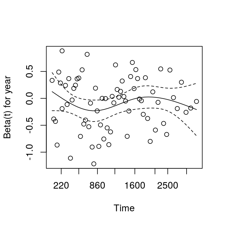
##           chisq df     p
## age       2.067  1 0.151
## sex       0.505  1 0.477
## thickness 2.837  1 0.092
## ulcer     4.325  1 0.038
## year      0.451  1 0.502
## GLOBAL    7.891  5 0.162
10.8.5 Stratified models
One approach to dealing with a violation of the proportional hazards assumption is to stratify by that variable.
Including a strata() term will result in a separate baseline hazard function being fit for each level in the stratification variable. It will be no longer possible to make direct inference on the effect associated with that variable.
This can be incorporated directly into the explanatory variable list.
explanatory <- c("age", "sex", "ulcer", "thickness",
               "strata(year)")
melanoma %>%
finalfit(dependent_os, explanatory)| Dependent: Surv(time, status_os) | all | HR (univariable) | HR (multivariable) | |
|---|---|---|---|---|
| Age (years) | Mean (SD) | 52.5 (16.7) | 1.03 (1.01-1.05, p<0.001) | 1.03 (1.01-1.05, p=0.002) |
| Sex | Female | 126 (100.0) |
|
|
| Male | 79 (100.0) | 1.93 (1.21-3.07, p=0.006) | 1.75 (1.06-2.87, p=0.027) | |
| Ulcerated tumour | No | 115 (100.0) |
|
|
| Yes | 90 (100.0) | 3.52 (2.14-5.80, p<0.001) | 2.61 (1.47-4.63, p=0.001) | |
| Tumour thickness (mm) | Mean (SD) | 2.9 (3.0) | 1.16 (1.10-1.23, p<0.001) | 1.08 (1.01-1.16, p=0.027) |
| strata(year) |
|
|