11.6 Check for associations between missing and observed data
In deciding whether data is MCAR or MAR, one approach is to explore patterns of missingness between levels of included variables. This is particularly important (we would say absolutely required) for a primary outcome measure / dependent variable.
Take for example “death”. When that outcome is missing it is often for a particular reason. For example, perhaps patients undergoing emergency surgery were less likely to have complete records compared with those undergoing planned surgery. And of course, death is more likely after emergency surgery.
missing_pairs() uses functions from the GGally package.
It produces pairs plots to show relationships between missing values and observed values in all variables.
explanatory <- c("age", "sex.factor",
                 "nodes", "obstruct.factor",
                 "smoking_mcar", "smoking_mar")
dependent <- "mort_5yr"
colon_s %>%
  missing_pairs(dependent, explanatory)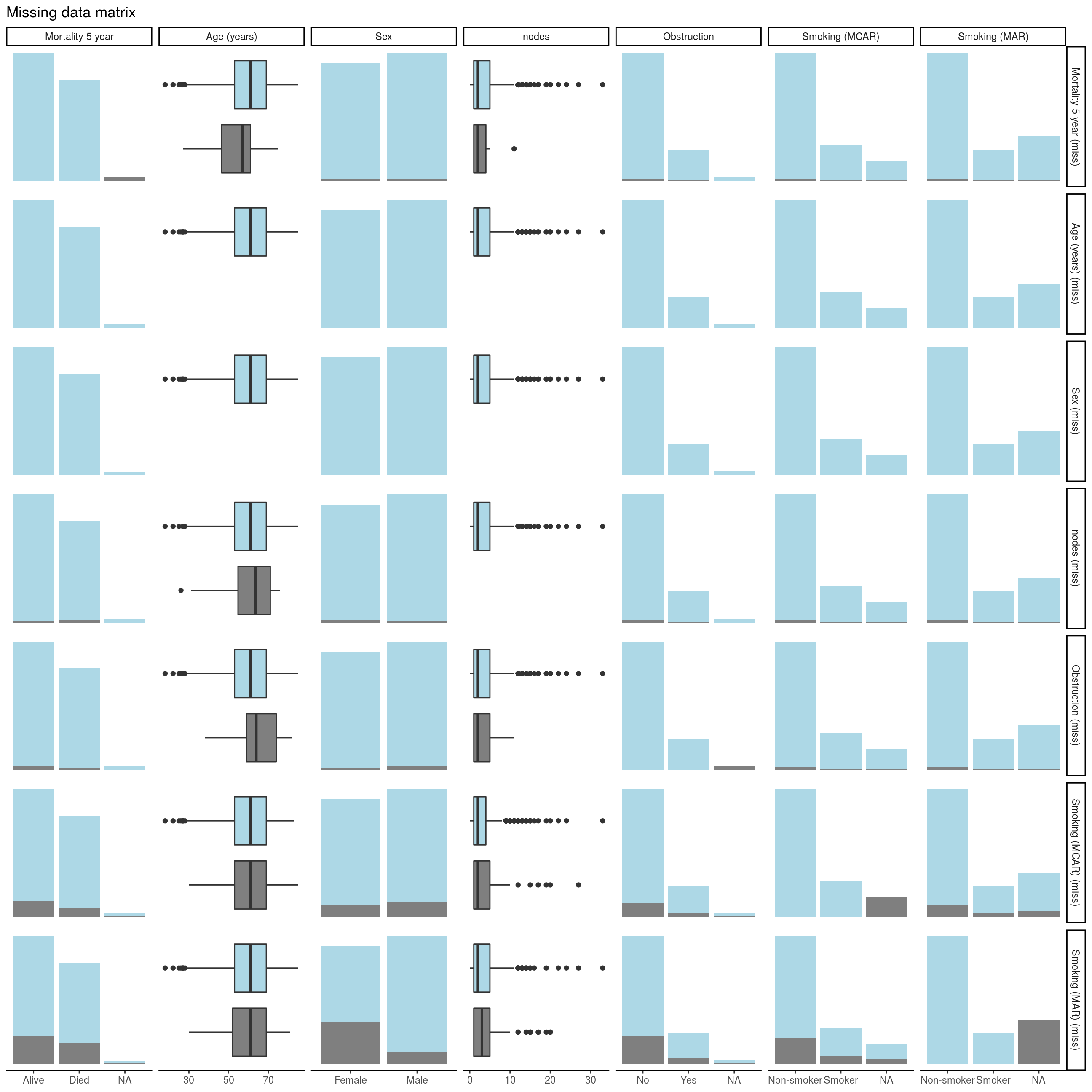
FIGURE 8.2: Missing data matrix with missing_pairs().
For continuous variables (age and nodes), the distributions of observed and missing data can immediately be visually compared. For example, look at Row 1 Column 2. The age of patients who’s mortality data is known is the blue box plot, and the age of patients with missing mortality data is the grey box plot.
For categorical data, the comparisons are presented as counts (remember geom_bar() from Chapter 4).
To be able to compare proportions, we can add the position = "fill" argument:
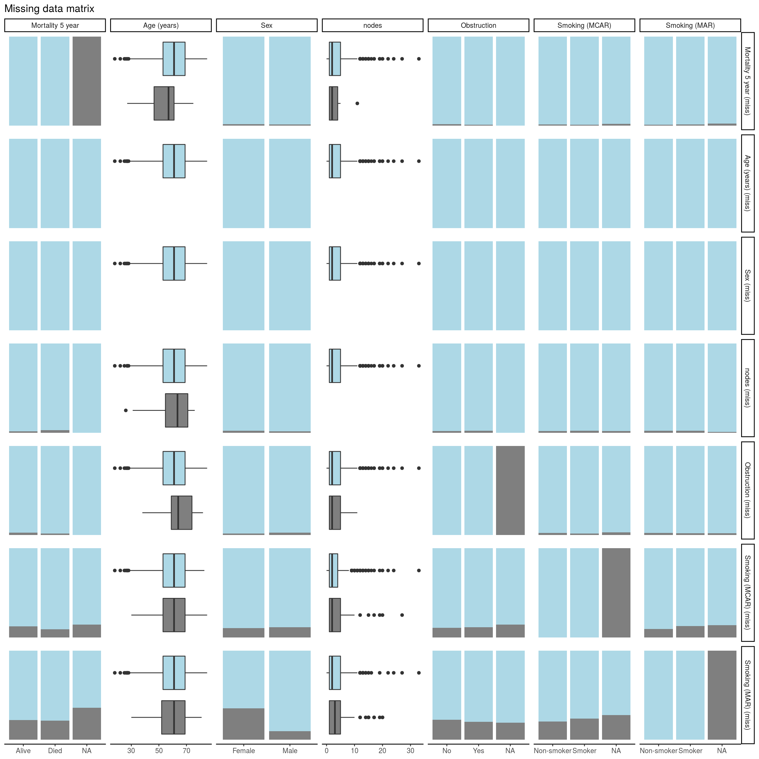
FIGURE 8.3: Missing data matrix with missing_pairs(position = 'fill') .
Find the two sets of bar plots that show the proportion of missing smoking data for sex (bottom of Column 3). Missingness in Smoking (MCAR) does not relate to sex - females and males have the same proportion of missing data. Missingness in Smoking (MAR), however, does differ by sex as females have more missing data than men here. This is how we designed the example at the top of this chapter, so it all makes sense.
We can also confirm this by using missing_compare():
explanatory <- c("age", "sex.factor",
                 "nodes", "obstruct.factor")
dependent <- "smoking_mcar"

missing_mcar <- colon_s %>%
missing_compare(dependent, explanatory)| Missing data analysis: Smoking (MCAR) | Not missing | Missing | p | |
|---|---|---|---|---|
| Age (years) | Mean (SD) | 59.7 (11.9) | 59.9 (12.6) | 0.882 |
| Sex | Female | 399 (89.7) | 46 (10.3) | 0.692 |
| Male | 429 (88.6) | 55 (11.4) | ||
| nodes | Mean (SD) | 3.6 (3.4) | 4.0 (4.5) | 0.302 |
| Obstruction | No | 654 (89.3) | 78 (10.7) | 0.891 |
| Yes | 156 (88.6) | 20 (11.4) |
| Missing data analysis: Smoking (MAR) | Not missing | Missing | p | |
|---|---|---|---|---|
| Age (years) | Mean (SD) | 59.9 (11.8) | 59.4 (12.6) | 0.632 |
| Sex | Female | 288 (64.7) | 157 (35.3) | <0.001 |
| Male | 438 (90.5) | 46 (9.5) | ||
| nodes | Mean (SD) | 3.6 (3.5) | 3.9 (3.9) | 0.321 |
| Obstruction | No | 568 (77.6) | 164 (22.4) | 0.533 |
| Yes | 141 (80.1) | 35 (19.9) |
It takes dependent and explanatory variables, and in this context “dependent” refers to the variable being tested for missingness against the explanatory variables.15 As expected, a relationship is seen between sex and smoking (MAR) but not smoking (MCAR).
11.6.1 For those who like an omnibus test
If you work predominately with continuous rather than categorical data, you may find these tests from the MissMech package useful.
It provides two tests which can be used to determine whether data are MCAR; the package and its output are well documented.
library(MissMech)
explanatory <- c("age", "nodes")
dependent <- "mort_5yr"

colon_s %>%
  select(all_of(explanatory)) %>%
  MissMech::TestMCARNormality()
## Call:
## MissMech::TestMCARNormality(data = .)
##
## Number of Patterns: 2
##
## Total number of cases used in the analysis: 929
##
## Pattern(s) used:
## age nodes Number of cases
## group.1 1 1 911
## group.2 1 NA 18
##
##
## Test of normality and Homoscedasticity:
## -------------------------------------------
##
## Hawkins Test:
##
## P-value for the Hawkins test of normality and homoscedasticity: 7.607252e-14
##
## Either the test of multivariate normality or homoscedasticity (or both) is rejected.
## Provided that normality can be assumed, the hypothesis of MCAR is
## rejected at 0.05 significance level.
##
## Non-Parametric Test:
##
## P-value for the non-parametric test of homoscedasticity: 0.6171955
##
## Reject Normality at 0.05 significance level.
## There is not sufficient evidence to reject MCAR at 0.05 significance level.By default,
missing_compare()uses an F-test test for continuous variables and chi-squared for categorical variables; you can change these the same way you change tests insummary_factorlist(). Check the Help tab or online documentation for a reminder.↩︎