13.8 PDF via knitr/R Markdown

Without changing anything in Example 1 and Knitting it into a PDF, we get 13.3A.

Again, most of it already looks pretty good, but some parts over-run the page and the plot is not a good size.

We can fix the plot in exactly the same way we did for the Word version (fig.width), but the second table that is too wide needs some special handling. For this we use kable_styling(font_size=8) from the kableExtra package. Remember to install it when using for the first time, and include library(knitExtra) alongside the other library lines at the setup chunk.

We will also alter the margins of your page using the geometry option in the preamble as the default margins of a PDF document coming out of R Markdown are a bit wide for us.

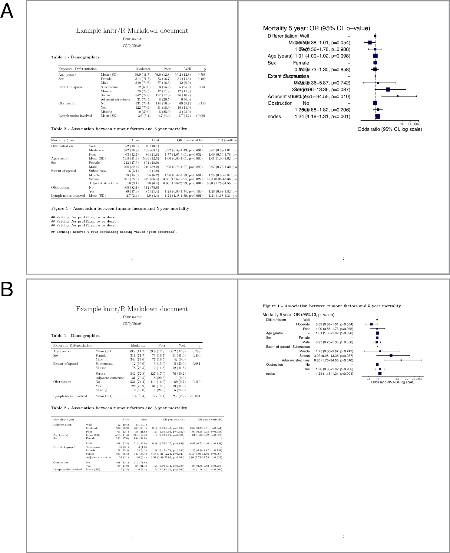
FIGURE 13.3: Knitting to Microsoft Word from R Markdown. Before (A) and after (B) adjustment.

---
title: "Example knitr/R Markdown document"
author: "Your name"
date: "22/5/2020"
output:
  pdf_document: default
geometry: margin=0.75in
---

```{r setup, include=FALSE}
# Load data into global environment. 
library(finalfit)
library(dplyr)
library(knitr)
library(kableExtra)
load(here::here("data", "out.rda"))
```

## Table 1 - Demographics
```{r table1, echo = FALSE}
kable(table1, row.names=FALSE, align=c("l", "l", "r", "r", "r", "r"),
      booktabs = TRUE)
```

## Table 2 - Association between tumour factors and 5 year mortality
```{r table2, echo = FALSE}
kable(table2, row.names=FALSE, align=c("l", "l", "r", "r", "r", "r"),
      booktabs=TRUE) %>% 
kable_styling(font_size=8)
```

## Figure 1 - Association between tumour factors and 5 year mortality
```{r figure1, echo=FALSE, message=FALSE, warning=FALSE, fig.width=10}
explanatory = c( "differ.factor", "age", "sex.factor", 
                "extent.factor", "obstruct.factor", 
                "nodes")
dependent = "mort_5yr"
colon_s %>% 
  or_plot(dependent, explanatory, 
          breaks = c(0.5, 1, 5, 10, 20, 30))
```

The result is shown in Figure 13.3B.