6.13 Solutions

Solution to Exercise 6.12.1:

## Make a histogram, Q-Q plot, and a box-plot for the life expectancy
## for a continent of your choice, but for all years. 
## Do the data appear normally distributed?

asia_data <- gapdata %>%                          
  filter(continent %in% c("Asia"))              

p1 <- asia_data %>%                              
  ggplot(aes(x = lifeExp)) + 
  geom_histogram(bins = 15)

p2 <- asia_data %>%                          
  ggplot(aes(sample = lifeExp)) +             # sample =  for Q-Q plot
  geom_qq() + 
  geom_qq_line(colour = "blue")

p3 <- asia_data %>%                              
  ggplot(aes(x = year, y = lifeExp)) +  
  geom_boxplot(aes(fill = factor(year))) +  # optional: year as factor
  geom_jitter(alpha = 0.4) +                    
  theme(legend.position = "none")               

library(patchwork)                              
p1 / p2 | p3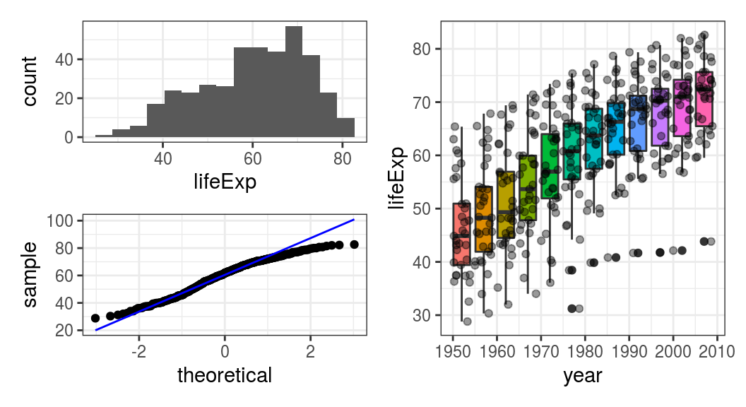

Solution to Exercise 6.12.2:

## Select any 2 years in any continent and perform a *t*-test to 
## determine whether mean life expectancy is significantly different. 
## Remember to plot your data first.

asia_2years <- asia_data %>%   
  filter(year %in% c(1952, 1972)) 

p1 <- asia_2years %>%   
  ggplot(aes(x = lifeExp)) + 
  geom_histogram(bins = 15) +                 
  facet_wrap(~year)                          

p2 <- asia_2years %>%   
  ggplot(aes(sample = lifeExp)) +              
  geom_qq() + 
  geom_qq_line(colour = "blue") + 
  facet_wrap(~year)                        

p3 <- asia_2years %>%         
  ggplot(aes(x = factor(year), y = lifeExp)) + 
  geom_boxplot(aes(fill = factor(year))) +      
  geom_jitter(alpha = 0.4) +                    
  theme(legend.position = "none")               

library(patchwork)                              
p1 / p2 | p3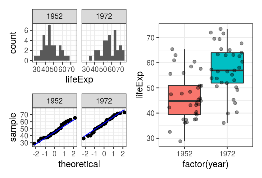

asia_2years %>% 
  t.test(lifeExp ~ year, data = .)

## 
##  Welch Two Sample t-test
## 
## data:  lifeExp by year
## t = -4.7007, df = 63.869, p-value = 1.428e-05
## alternative hypothesis: true difference in means is not equal to 0
## 95 percent confidence interval:
##  -15.681981  -6.327769
## sample estimates:
## mean in group 1952 mean in group 1972 
##           46.31439           57.31927

Solution to Exercise 6.12.3:

## In 2007, in which continents did mean life expectancy differ from 70
gapdata %>% 
  filter(year == 2007) %>% 
  group_by(continent) %>%
  do(
    t.test(.$lifeExp, mu = 70) %>%
      tidy()                         
  )

## # A tibble: 5 x 9
## # Groups:   continent [5]
##   continent estimate statistic  p.value parameter conf.low conf.high method
##   <fct>        <dbl>     <dbl>    <dbl>     <dbl>    <dbl>     <dbl> <chr> 
## 1 Africa        54.8   -11.4   1.33e-15        51     52.1      57.5 One S…
## 2 Americas      73.6     4.06  4.50e- 4        24     71.8      75.4 One S…
## 3 Asia          70.7     0.525 6.03e- 1        32     67.9      73.6 One S…
## 4 Europe        77.6    14.1   1.76e-14        29     76.5      78.8 One S…
## 5 Oceania       80.7    20.8   3.06e- 2         1     74.2      87.3 One S…
## # … with 1 more variable: alternative <chr>

Solution to Exercise 6.12.4:

## Use Kruskal-Wallis to determine if the mean population changed 
## significantly through the 1990s/2000s in individual continents. 

gapdata %>% 
  filter(year >= 1990) %>% 
  ggplot(aes(x = factor(year), y = pop)) + 
  geom_boxplot() + 
  facet_wrap(~continent)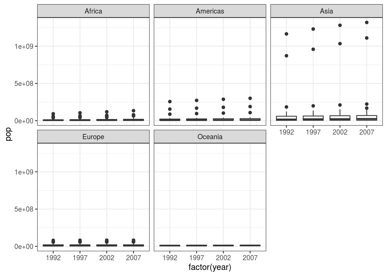

gapdata %>% 
  filter(year >= 1990) %>% 
  group_by(continent) %>% 
  do(
    kruskal.test(pop ~ year, data = .) %>%
      tidy()
  )

## # A tibble: 5 x 5
## # Groups:   continent [5]
##   continent statistic p.value parameter method                      
##   <fct>         <dbl>   <dbl>     <int> <chr>                       
## 1 Africa        2.10    0.553         3 Kruskal-Wallis rank sum test
## 2 Americas      0.847   0.838         3 Kruskal-Wallis rank sum test
## 3 Asia          1.57    0.665         3 Kruskal-Wallis rank sum test
## 4 Europe        0.207   0.977         3 Kruskal-Wallis rank sum test
## 5 Oceania       1.67    0.644         3 Kruskal-Wallis rank sum test