5.2 Scales

5.2.1 Logarithmic

Transforming an axis to a logarithmic scale can be done by adding on scale_x_log10():

p1 <- p0 + scale_x_log10()

scale_x_log10() and scale_x_log10() are shortcuts for the base-10 logarithmic transformation of an axis. The same could be achieved by using, e.g., scale_x_continuous(trans = "log10"). The latter can take a selection of options, namely "reverse", "log2", or "sqrt". Check the Help tab for scale_continuous() or look up its online documentation for a full list.

5.2.2 Expand limits

A quick way to expand the limits of your plot is to specify the value you want to be included:

p2 <- p0 + expand_limits(y = 0)

Or two values for extending to both sides of the plot:

p3 <- p0 + expand_limits(y = c(0, 100))

By default, ggplot() adds some padding around the included area (see how the scale doesn’t start from 0, but slightly before). This ensures points on the edges don’t get overlapped with the axes, but in some cases - especially if you’ve already expanded the scale, you might want to remove this extra padding. You can remove this padding with the expand argument:

p4 <- p0 +
  expand_limits(y = c(0, 100)) +
  coord_cartesian(expand = FALSE)

We are now using a new library - patchwork - to print all 4 plots together (Figure 5.2). Its syntax is very simple - it allows us to add ggplot objects together. (Trying to do p1 + p2 without loading the patchwork package will not work, R will say “Error: Don’t know how to add p2 to a plot”.)

library(patchwork)
p1 + p2 + p3 + p4 + plot_annotation(tag_levels = "1", tag_prefix = "p")

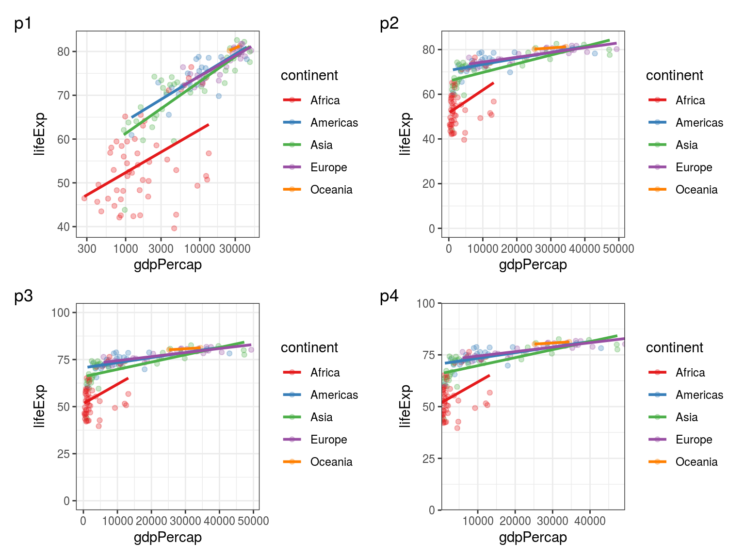
FIGURE 5.2: p1: Using a logarithmic scale for the x axis. p2: Expanding the limits of the y axis to include 0. p3: Expanding the limits of the y axis to include 0 and 100. p4: Removing extra padding around the limits.

5.2.3 Zoom in

p5 <- p0 +
  coord_cartesian(ylim = c(70, 85), xlim = c(20000, 40000)) 

5.2.4 Exercise

How is this one different to the previous (Figure 5.3)?

p6 <- p0 +
  scale_y_continuous(limits = c(70, 85)) +
  scale_x_continuous(limits = c(20000, 40000)) 

Answer: the first one zooms in, still retaining information about the excluded points when calculating the linear regression lines. The second one removes the data (as the warnings say), calculating the linear regression lines only for the visible points.

p5 + labs(tag = "p5") + p6 + labs(tag = "p6")

## Warning: Removed 114 rows containing non-finite values (stat_smooth).

## Warning: Removed 114 rows containing missing values (geom_point).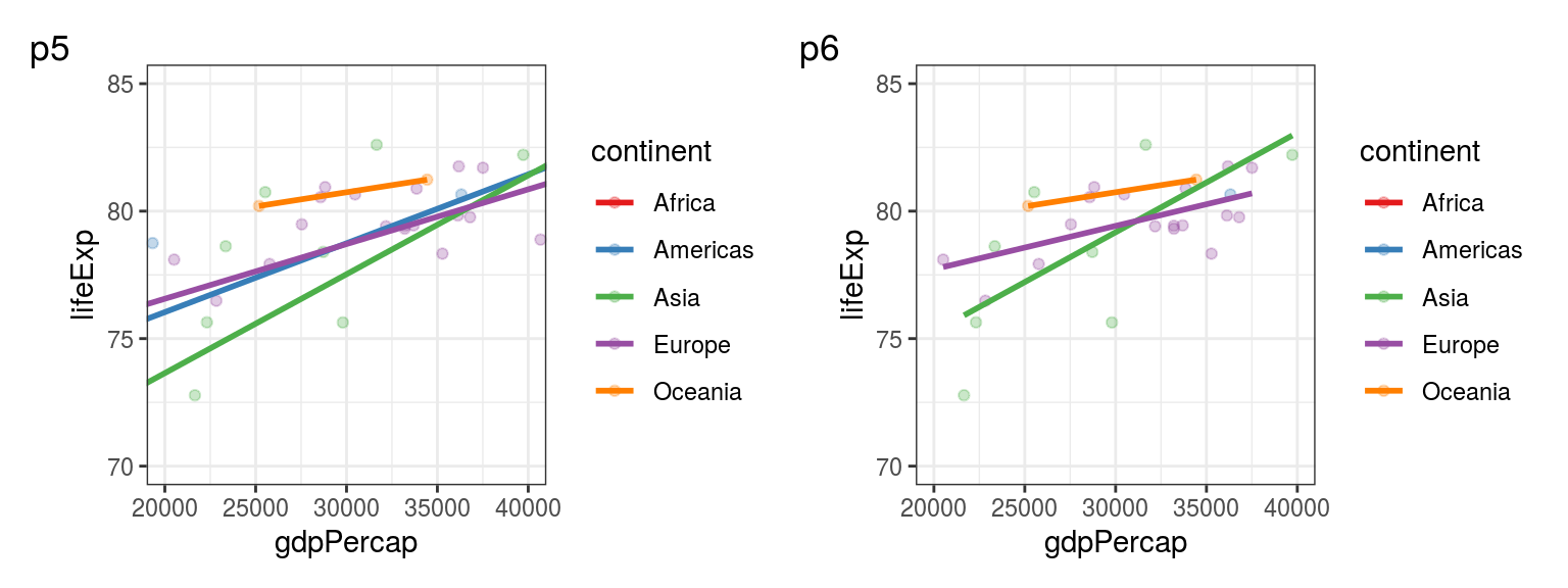

FIGURE 5.3: p5: Using coord_cartesian() vs p6: Using scale_x_continuous() and scale_y_continuous() for setting the limits of plot axes.

Preivously we used patchwork’s plot_annotation() function to create our multiplot tags. Since our exmaples no longer start the count from 1, we’re using ggplot()’s tags instead, e.g., labs(tag = "p5"). The labs() function iwill be covered in more detail later in this chapter.

5.2.5 Axis ticks

ggplot() does a good job deciding how many and which values include on the axis (e.g., 70/75/80/85 for the y axes in Figure 5.3). But sometimes you’ll want to specify these, for example, to indicate threshold values or a maximum (Figure 5.4). We can do so by using the breaks argument:

# calculating the maximum value to be included in the axis breaks:
max_value = gapminder %>% 
  filter(year == 2007) %>%
  summarise(max_lifeExp = max(lifeExp)) %>% 
  pull(max_lifeExp) %>% 
  round(1)

# using scale_y_continuous(breaks = ...):
p7 <-  p0 +
  coord_cartesian(ylim = c(0, 100), expand = 0) +
  scale_y_continuous(breaks = c(18, 50, max_value))

# we may also include custom labels for our breaks:
p8 <-  p0 +
  coord_cartesian(ylim = c(0, 100), expand = 0) +
  scale_y_continuous(breaks = c(18, 50, max_value), labels = c("Adults", "50", "MAX"))

p7 + labs(tag = "p7") + p8 + labs(tag = "p8")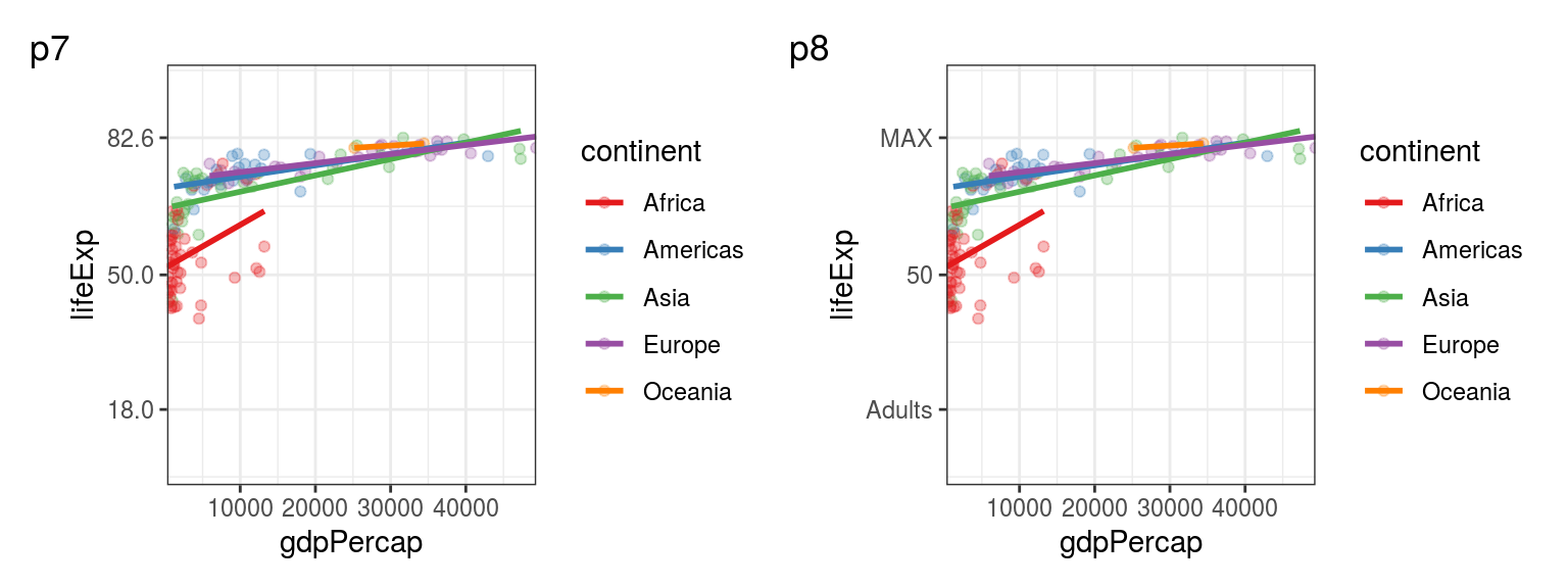

FIGURE 5.4: p7: Specifiying y axis breaks. p8: Adding custom labels for our breaks.