9.9 Correlated groups of observations
In our modelling strategy above, we mentioned the incorporation of population stratification if available. What does this mean?
Our regression is seeking to capture the characteristics of particular patients. These characteristics are made manifest through the slopes of fitted lines - the estimated coefficients (ORs) of particular variables. A goal is to estimate these characteristics as precisely as possible. Bias can be introduced when correlations between patients are not accounted for. Correlations may be as simple as being treated within the same hospital. By virtue of this fact, these patients may have commonalities that have not been captured by the observed variables.
Population characteristics can be incorporated into our models. We may not be interested in capturing and measuring the effects themselves, but want to ensure they are accounted for in the analysis.
One approach is to include grouping variables as random effects.
These may be nested with each other, for example patients within hospitals within countries.
These are added in addition to the fixed effects we have been dealing with up until now.
These models go under different names including mixed effects model, multilevel model, or hierarchical model.
Other approaches, such as generalized estimating equations are not dealt with here.
9.9.1 Simulate data
Our melanoma dataset doesn’t include any higher level structure, so we will simulate this for demonstration purposes. We have just randomly allocated 1 of 4 identifiers to each patient below.
9.9.2 Plot the data
We will speak in terms of ‘hospitals’ now, but the grouping variable(s) could clearly be anything.
The simplest random effects approach is a ‘random intercept model’. This allows the intercept of fitted lines to vary by hospital. The random intercept model constrains lines to be parallel, in a similar way to the additive models discussed above and in Chapter 7.
It is harder to demonstrate with binomial data, but we can stratify the 5-year mortality by T-stage (considered as a continuous variable for this purpose). Note there were no deaths in ‘hospital 4’ (Figure 9.14). We can model this accounting for inter-hospital variation below.
melanoma %>%
    mutate(
    mort_5yr.num = as.numeric(mort_5yr) - 1 # Convert factor to 0 and 1
  ) %>%
  ggplot(aes(x = as.numeric(t_stage.factor), y = mort_5yr.num)) +
  geom_jitter(width = 0.1, height = 0.1) +
  geom_smooth(method = 'loess', se = FALSE) +
  facet_wrap(~hospital_id) +
  labs(x= "T-stage", y = "Mortality (5 y)")
## `geom_smooth()` using formula 'y ~ x'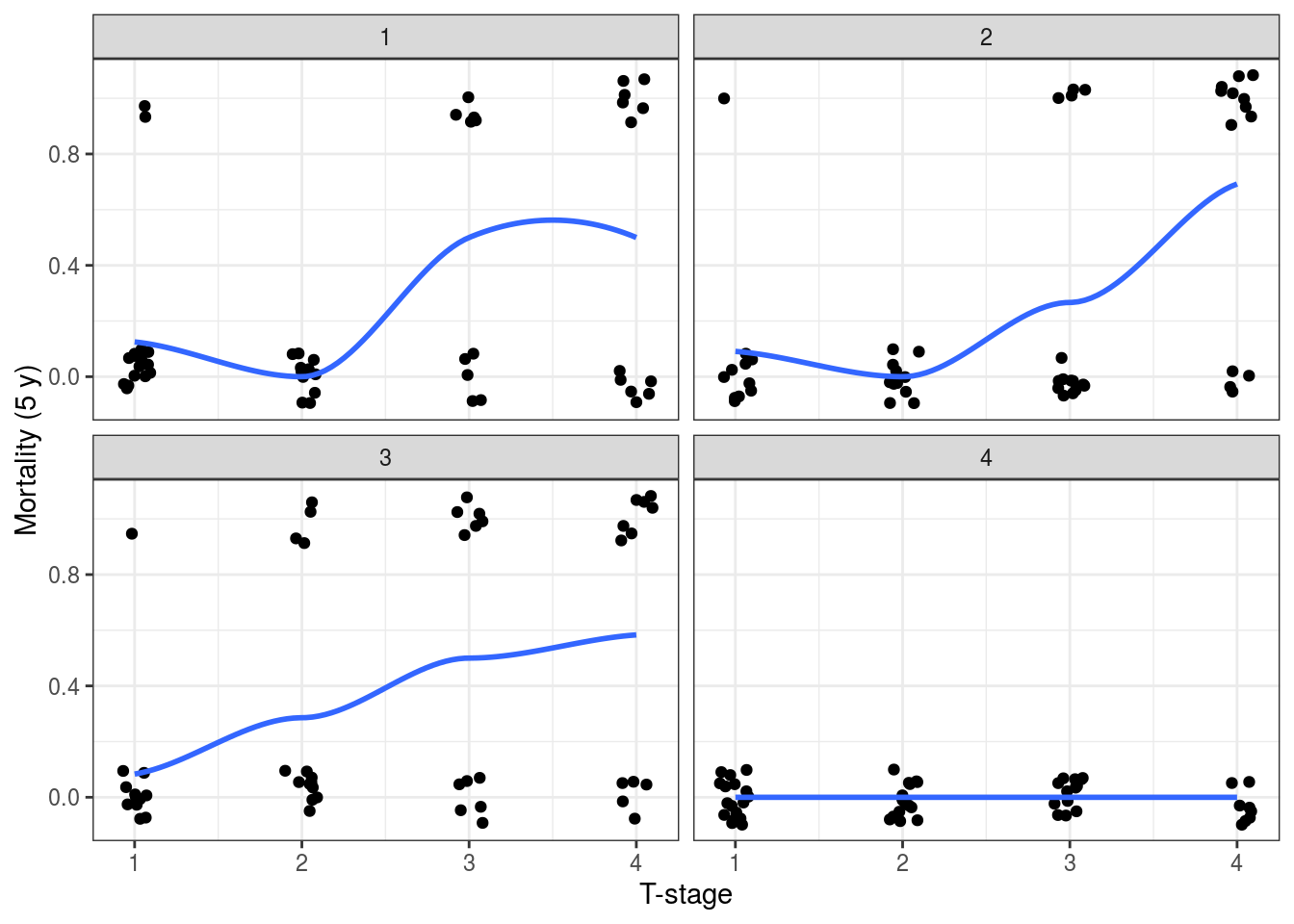
FIGURE 9.14: Investigating random effects by looking at the relationship between the outcome variable (5-year mortality) and T-stage at each hospital.
9.9.3 Mixed effects models in base R
There are a number of different packages offering mixed effects modelling in R, our preferred is lme4.
## Loading required package: Matrix##
## Attaching package: 'Matrix'## The following objects are masked from 'package:tidyr':
##
## expand, pack, unpack## Registered S3 methods overwritten by 'lme4':
## method from
## cooks.distance.influence.merMod car
## influence.merMod car
## dfbeta.influence.merMod car
## dfbetas.influence.merMod carmelanoma %>%
glmer(mort_5yr ~ t_stage.factor + (1 | hospital_id),
data = ., family = "binomial") %>%
summary()## Generalized linear mixed model fit by maximum likelihood (Laplace
## Approximation) [glmerMod]
## Family: binomial ( logit )
## Formula: mort_5yr ~ t_stage.factor + (1 | hospital_id)
## Data: .
##
## AIC BIC logLik deviance df.resid
## 174.6 191.2 -82.3 164.6 200
##
## Scaled residuals:
## Min 1Q Median 3Q Max
## -1.4507 -0.3930 -0.2891 -0.0640 3.4591
##
## Random effects:
## Groups Name Variance Std.Dev.
## hospital_id (Intercept) 2.619 1.618
## Number of obs: 205, groups: hospital_id, 4
##
## Fixed effects:
## Estimate Std. Error z value Pr(>|z|)
## (Intercept) -3.13132 1.01451 -3.087 0.00203 **
## t_stage.factorT2 0.02256 0.74792 0.030 0.97593
## t_stage.factorT3 1.82349 0.62920 2.898 0.00375 **
## t_stage.factorT4 2.61190 0.62806 4.159 3.2e-05 ***
## ---
## Signif. codes: 0 '***' 0.001 '**' 0.01 '*' 0.05 '.' 0.1 ' ' 1
##
## Correlation of Fixed Effects:
## (Intr) t_s.T2 t_s.T3
## t_stg.fctT2 -0.365
## t_stg.fctT3 -0.454 0.591
## t_stg.fctT4 -0.459 0.590 0.718The base R output is similar to glm().
It includes the standard deviation on the random effects intercept as well.
Meaning the variation between hospitals being captured by the model.
The output can be examined using tidy() and glance() functions as above.
We find it more straightforward to use finalfit.
dependent <- "mort_5yr"
explanatory <- "t_stage.factor"
random_effect <- "hospital_id" # Is the same as:
random_effect <- "(1 | hospital_id)"
melanoma %>%
  finalfit(dependent, explanatory,
           random_effect = random_effect,
           metrics = TRUE)
We can incorporate our (made-up) hospital identifier into our final model from above.
Using keep_models = TRUE, we can compare univariable, multivariable and mixed effects models.
library(finalfit)
dependent <- "mort_5yr"
explanatory <- c("ulcer.factor", "age.factor",
                "sex.factor", "t_stage.factor")
explanatory_multi <- c("ulcer.factor", "t_stage.factor")
random_effect <- "hospital_id"
melanoma %>%
  finalfit(dependent, explanatory, explanatory_multi, random_effect,
           keep_models = TRUE,
metrics = TRUE)| Dependent: 5-year survival | No | Yes | OR (univariable) | OR (multivariable) | OR (multivariable reduced) | OR (multilevel) | |
|---|---|---|---|---|---|---|---|
| Ulcerated tumour | Absent | 105 (91.3) | 10 (8.7) |
|
|
|
|
| Present | 55 (61.1) | 35 (38.9) | 6.68 (3.18-15.18, p<0.001) | 3.06 (1.25-7.93, p=0.017) | 3.26 (1.35-8.39, p=0.011) | 2.49 (0.94-6.59, p=0.065) | |
| Age (years) | (0,25] | 10 (71.4) | 4 (28.6) |
|
|
|
|
| (25,50] | 62 (84.9) | 11 (15.1) | 0.44 (0.12-1.84, p=0.229) | 0.37 (0.08-1.80, p=0.197) |
|
|
|
| (50,75] | 79 (76.0) | 25 (24.0) | 0.79 (0.24-3.08, p=0.712) | 0.60 (0.15-2.65, p=0.469) |
|
|
|
| (75,100] | 9 (64.3) | 5 (35.7) | 1.39 (0.28-7.23, p=0.686) | 0.61 (0.09-4.04, p=0.599) |
|
|
|
| Sex | Female | 105 (83.3) | 21 (16.7) |
|
|
|
|
| Male | 55 (69.6) | 24 (30.4) | 2.18 (1.12-4.30, p=0.023) | 1.21 (0.54-2.68, p=0.633) |
|
|
|
| T-stage | T1 | 52 (92.9) | 4 (7.1) |
|
|
|
|
| T2 | 49 (92.5) | 4 (7.5) | 1.06 (0.24-4.71, p=0.936) | 0.74 (0.15-3.50, p=0.697) | 0.75 (0.16-3.45, p=0.700) | 0.83 (0.18-3.73, p=0.807) | |
| T3 | 36 (70.6) | 15 (29.4) | 5.42 (1.80-20.22, p=0.005) | 2.91 (0.84-11.82, p=0.106) | 2.96 (0.86-11.96, p=0.098) | 3.83 (1.00-14.70, p=0.051) | |
| T4 | 23 (51.1) | 22 (48.9) | 12.43 (4.21-46.26, p<0.001) | 5.38 (1.43-23.52, p=0.016) | 5.33 (1.48-22.56, p=0.014) | 7.03 (1.71-28.86, p=0.007) |
| Number in dataframe = 205, Number in model = 205, Missing = 0, AIC = 190, C-statistic = 0.802, H&L = Chi-sq(8) 13.87 (p=0.085) |
| Number in dataframe = 205, Number in model = 205, Missing = 0, AIC = 184.4, C-statistic = 0.791, H&L = Chi-sq(8) 0.43 (p=1.000) |
| Number in model = 205, Number of groups = 4, AIC = 173.2, C-statistic = 0.866 |
As can be seen, incorporating the (made-up) hospital identifier has altered our coefficients.
It has also improved the model discrimination with a c-statistic of 0.830 from 0.802.
Note that the AIC should not be used to compare mixed effects models estimated in this way with glm() models (the former uses a restricted maximum likelihood [REML] approach by default, while glm() uses maximum likelihood).
Random slope models are an extension of the random intercept model.
Here the gradient of the response to a particular variable is allowed to vary by hospital.
For example, this can be included using random_effect = "(thickness | hospital_id)" where the gradient of the continuous variable tumour thickness was allow to vary by hospital.
As models get more complex, care has to be taken to ensure the underlying data is understood and assumptions are checked.
Mixed effects modelling is a book in itself and the purpose here is to introduce the concept and provide some approaches for its incorporation. Clearly much is written elsewhere for those who are enthusiastic to learn more.