9.4 Model assumptions
Binary logistic regression is robust to many of the assumptions which cause problems in other statistical analyses. The main assumptions are:
- Binary dependent variable - this is obvious, but as above we need to check (alive, death from disease, death from other causes doesn’t work);
- Independence of observations - the observations should not be repeated measurements or matched data;
- Linearity of continuous explanatory variables and the log-odds outcome - take age as an example. If the outcome, say death, gets more frequent or less frequent as age rises, the model will work well. However, say children and the elderly are at high risk of death, but those in middle years are not, then the relationship is not linear. Or more correctly, it is not monotonic, meaning that the response does not only go in one direction;
- No multicollinearity - explanatory variables should not be highly correlated with each other.
9.4.1 Linearity of continuous variables to the response
A graphical check of linearity can be performed using a best fit “loess” line. This is on the probability scale, so it is not going to be straight. But it should be monotonic - it should only ever go up or down.
melanoma %>%
  mutate(
    mort_5yr.num = as.numeric(mort_5yr) - 1
  ) %>%
  select(mort_5yr.num, age, year) %>%
  pivot_longer(all_of(c("age", "year")), names_to = "predictors") %>%
  ggplot(aes(x = value, y = mort_5yr.num)) +
  geom_point(size = 0.5, alpha = 0.5) +
  geom_smooth(method = "loess") +
  facet_wrap(~predictors, scales = "free_x")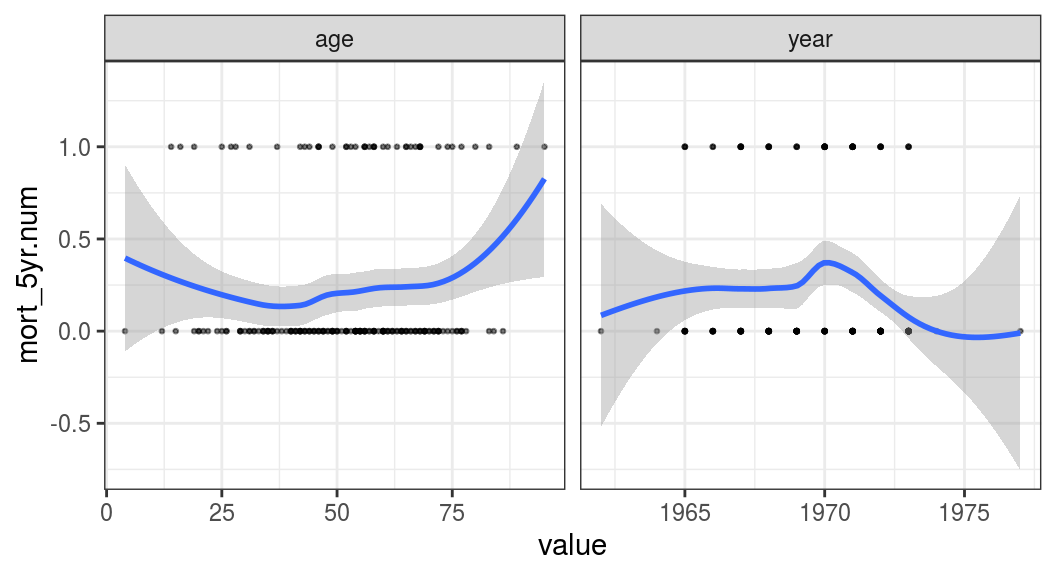
FIGURE 9.9: Linearity of our continuous explanatory variables to the outcome (5-year mortality).
Figure 9.9 shows that age is interesting as the relationship is u-shaped. The chance of death is higher in the young and the old compared with the middle-aged. This will need to be accounted for in any model including age as a predictor.
9.4.2 Multicollinearity
The presence of two or more highly correlated variables in a regression analysis can cause problems in the results which are generated. The slopes of lines (coefficients, ORs) can become unstable, which means big shifts in their size with minimal changes to the model or the underlying data. The confidence intervals around these coefficients may also be large. Definitions of the specifics differ between sources, but there are broadly two situations.
The first is when two highly correlated variables have been included in a model, sometimes referred to simply as collinearity. This can be detected by thinking about which variables may be correlated, and then checking using plotting.
The second situation is more devious. It is where collinearity exists between three or more variables, even when no pair of variables is particularly highly correlated. To detect this, we can use a specific metric called the variance inflation factor.
As always though, think clearly about your data and whether there may be duplication of information. Have you included a variable which is calculated from other variables already included in the model? Including body mass index (BMI), weight and height would be problematic, given the first is calculated from the latter two.
Are you describing a similar piece of information in two different ways? For instance, all perforated colon cancers are staged T4, so do you include T-stage and the perforation factor? (Note, not all T4 cancers have perforated.)
The ggpairs() function from library(GGally) is a good way of visualising all two-way associations (Figure 9.10).
library(GGally)
explanatory <- c("ulcer.factor", "age", "sex.factor",
                "year", "t_stage.factor")
melanoma %>%
  remove_labels() %>%  # ggpairs doesn't work well with labels
  ggpairs(columns = explanatory)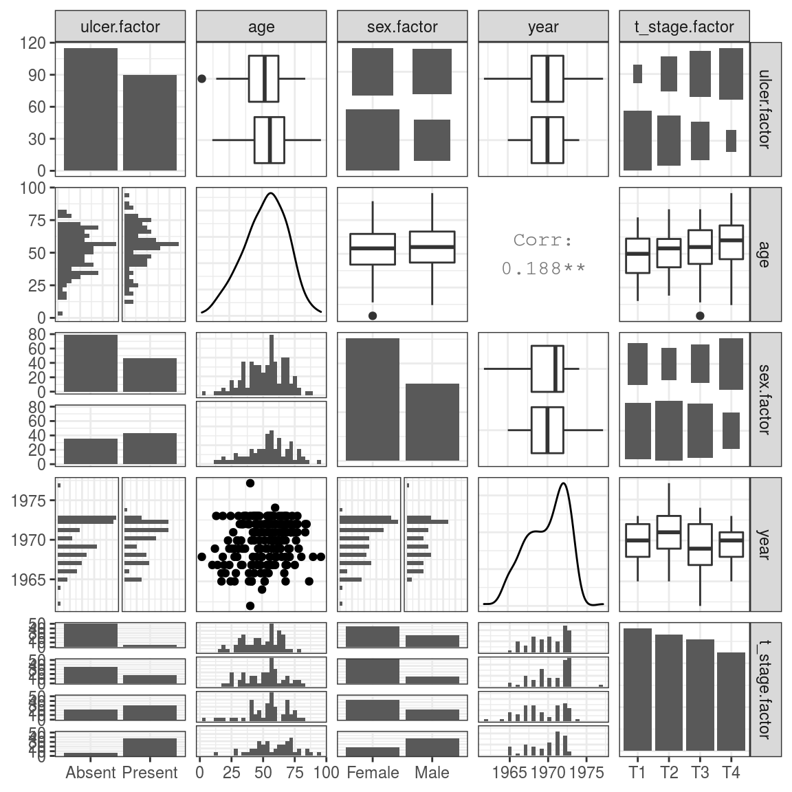
FIGURE 9.10: Exploring two-way associations within our explanatory variables.
If you have many variables you want to check you can split them up.
Continuous to continuous
Here we’re using the same library(GGally) code as above, but shortlisting the two categorical variables: age and year (Figure 9.11):
select_explanatory <- c("age", "year")
melanoma %>%
  remove_labels() %>%
  ggpairs(columns = select_explanatory)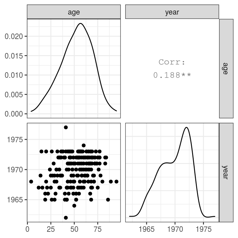
FIGURE 9.11: Exploring relationships between continuous variables.
Continuous to categorical
Let’s use a clever pivot_longer() and facet_wrap() combination to efficiently plot multiple variables against each other without using ggpairs().
We want to compare everything against, for example, age so we need to include -age in the pivot_longer() call so it doesn’t get lumped up with everything else (Figure 9.12):
select_explanatory <- c("age", "ulcer.factor",
                       "sex.factor", "t_stage.factor")

melanoma %>%
  select(all_of(select_explanatory)) %>%
  pivot_longer(-age) %>% # pivots all but age into two columns: name and value
  ggplot(aes(value, age)) +
  geom_boxplot() +
  facet_wrap(~name, scale = "free", ncol = 3) +
  coord_flip()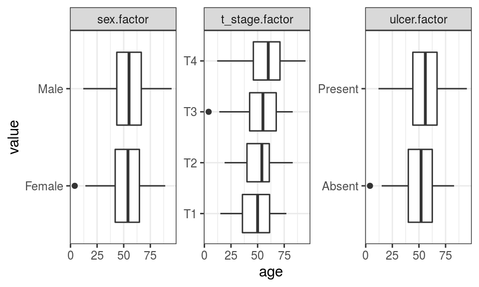
FIGURE 9.12: Exploring associations between continuous and categorical explanatory variables.
Categorical to categorical
select_explanatory <- c("ulcer.factor", "sex.factor", "t_stage.factor")

melanoma %>%
  select(one_of(select_explanatory)) %>%
  pivot_longer(-sex.factor) %>%
  ggplot(aes(value, fill = sex.factor)) +
  geom_bar(position = "fill") +
  ylab("proportion") +
  facet_wrap(~name, scale = "free", ncol = 2) +
  coord_flip()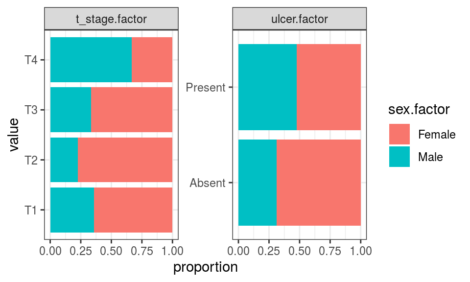
None of the explanatory variables are highly correlated with one another.
Variance inflation factor
Finally, as a final check for the presence of higher-order correlations, the variance inflation factor can be calculated for each of the terms in a final model. In simple language, this is a measure of how much the variance of a particular regression coefficient is increased due to the presence of multicollinearity in the model.
Here is an example. GVIF stands for generalised variance inflation factor. A common rule of thumb is that if this is greater than 5-10 for any variable, then multicollinearity may exist. The model should be further explored and the terms removed or reduced.
dependent <- "mort_5yr"
explanatory <- c("ulcer.factor", "age", "sex.factor",
                "year", "t_stage.factor")
melanoma %>%
  glmmulti(dependent, explanatory) %>%
  car::vif()
## GVIF Df GVIF^(1/(2*Df))
## ulcer.factor 1.313355 1 1.146017
## age 1.102313 1 1.049911
## sex.factor 1.124990 1 1.060655
## year 1.102490 1 1.049995
## t_stage.factor 1.475550 3 1.066987We are not trying to over-egg this, but multicollinearity can be important. The message as always is the same. Understand the underlying data using plotting and tables, and you are unlikely to come unstuck.