10.13 Solutions
Solution to Exercise 10.12.1:
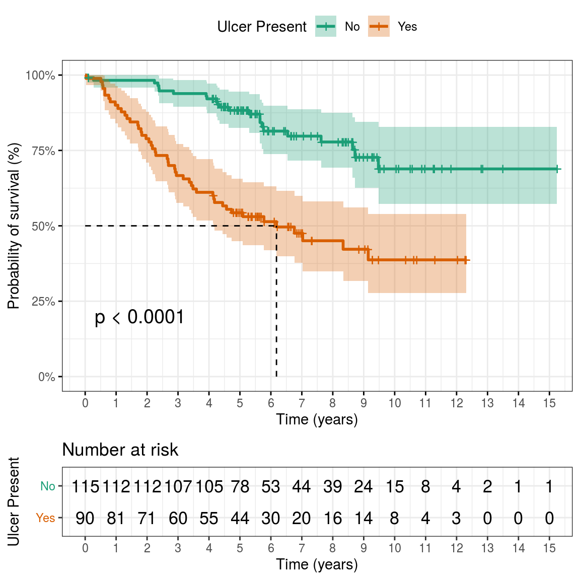
## Call: survfit(formula = survival_object ~ ulcer, data = melanoma)
##
##                 ulcer=No
##  time n.risk n.event survival std.err lower 95% CI upper 95% CI
##     0    115       0    1.000  0.0000        1.000        1.000
##     1    112       2    0.983  0.0122        0.959        1.000
##     2    112       0    0.983  0.0122        0.959        1.000
##     3    107       5    0.939  0.0225        0.896        0.984
##     4    105       2    0.921  0.0252        0.873        0.972
##     5     78       4    0.883  0.0306        0.825        0.945
##
##                 ulcer=Yes
##  time n.risk n.event survival std.err lower 95% CI upper 95% CI
##     0     90       0    1.000  0.0000        1.000        1.000
##     1     81       9    0.900  0.0316        0.840        0.964
##     2     71      10    0.789  0.0430        0.709        0.878
##     3     60      11    0.667  0.0497        0.576        0.772
##     4     55       5    0.611  0.0514        0.518        0.721
##     5     44       6    0.543  0.0526        0.449        0.657
## Warning: Vectorized input to `element_text()` is not officially supported.
## Results may be unexpected or may change in future versions of ggplot2.
Solution to Exercise 10.12.2:
# Fit model
my_hazard = coxph(survival_object ~ sex + ulcer + age + thickness, data=melanoma)
summary(my_hazard)

# Melanoma thickness has a HR 1.11 (1.03 to 1.18).
# This is interpretted as a 11% increase in the
# risk of death at any time for each 1 mm increase in thickness.

# Check assumptions
ph = cox.zph(my_hazard)
ph
# GLOBAL shows no overall violation of assumptions.
# Plot Schoenfield residuals to evaluate PH
plot(ph, var=4)We also include a section on dealing with missing data in R. Something that we both feel strongly about and which is often poorly described and dealt with in academic publishing.