8.6 Should I convert a continuous variable to a categorical variable?

This is a common question and something which is frequently done. Take for instance the variable age. Is it better to leave it as a continuous variable, or to chop it into categories, e.g., 30 to 39 etc.?

The clear disadvantage in doing this is that information is being thrown away. Which feels like a bad thing to be doing. This is particularly important if the categories being created are large.

For instance, if age was dichotomised to “young” and “old” at say 42 years (the current median age in Europe), then it is likely that relevant information to a number of analyses has been discarded.

Secondly, it is unforgivable practice to repeatedly try different cuts of a continuous variable to obtain a statistically significant result. This is most commonly done in tests of diagnostic accuracy, where a threshold for considering a continuous test result positive is chosen post hoc to maximise sensitivity/specificity, but not then validated in an independent cohort.

But there are also advantages to converting a continuous variable to categorical. Say the relationship between age and an outcome is not linear, but rather u-shaped, then fitting a regression line is more difficult. If age is cut into 10-year bands and entered into a regression as a factor, then this non-linearity is already accounted for.

Secondly, when communicating the results of an analysis to a lay audience, it may be easier to use a categorical representation. For instance, an odds of death 1.8 times greater in 70-year-olds compared with 40-year-olds may be easier to grasp than a 1.02 times increase per year.

So what is the answer? Do not do it unless you have to. Plot and understand the continuous variable first. If you do it, try not to throw away too much information. Repeat your analyses both with the continuous data and categorical data to ensure there is no difference in the conclusion (often called a sensitivity analysis).

# Summary of age
meldata$age %>% 
  summary()

##    Min. 1st Qu.  Median    Mean 3rd Qu.    Max. 
##    4.00   42.00   54.00   52.46   65.00   95.00

meldata %>% 
  ggplot(aes(x = age)) + 
  geom_histogram()

## `stat_bin()` using `bins = 30`. Pick better value with `binwidth`.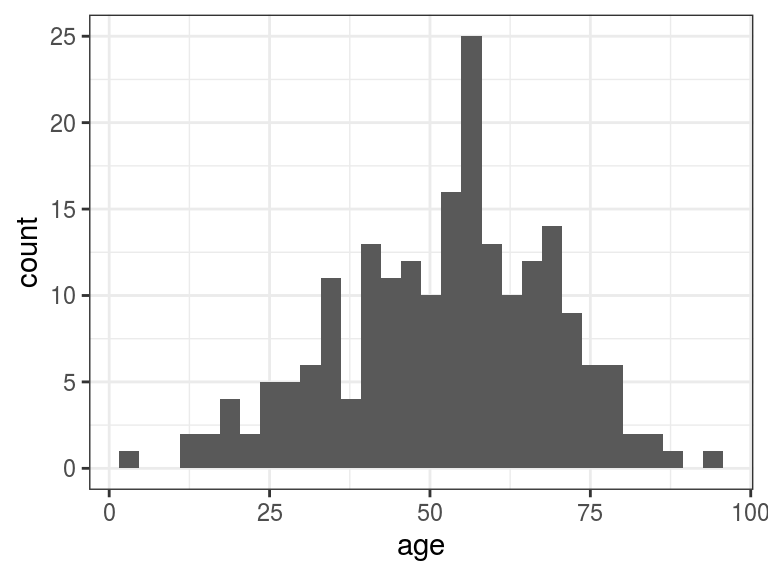

There are different ways in which a continuous variable can be converted to a factor. You may wish to create a number of intervals of equal length. The cut() function can be used for this.

Figure 8.1 illustrates different options for this. We suggest not using the label option of the cut() function to avoid errors, should the underlying data change or when the code is copied and reused. A better practice is to recode the levels using fct_recode as above.

The intervals in the output are standard mathematical notation. A square bracket indicates the value is included in the interval and a round bracket that the value is excluded.

Note the requirement for include.lowest = TRUE when you specify breaks yourself and the lowest cut-point is also the lowest data value. This should be clear in Figure 8.1.

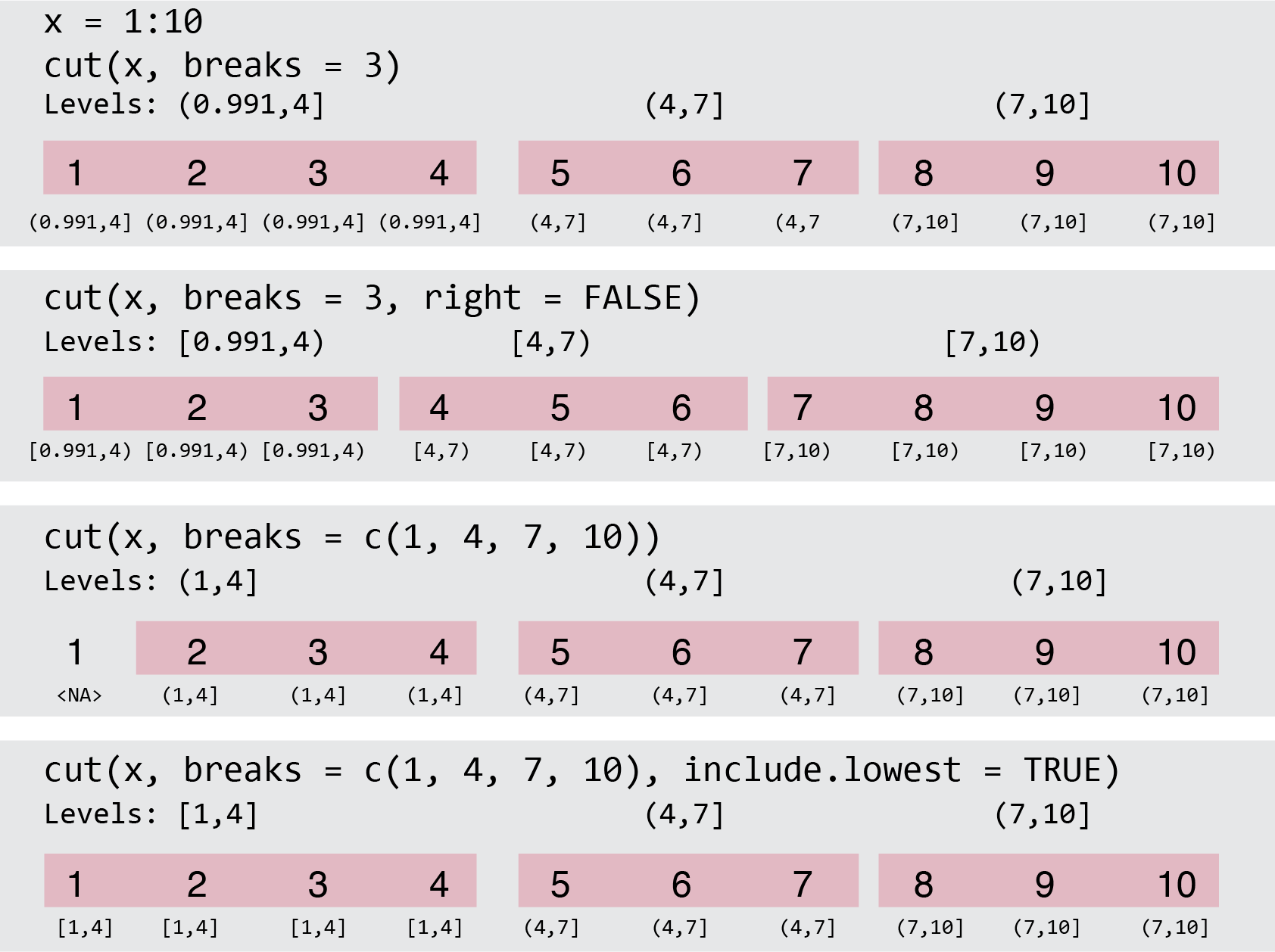
FIGURE 8.1: Cut a continuous variable into a categorical variable.

8.6.1 Equal intervals vs quantiles

Be clear in your head whether you wish to cut the data so the intervals are of equal length. Or whether you wish to cut the data so there are equal proportions of cases (patients) in each level.

Equal intervals:

meldata <- meldata %>% 
  mutate(
    age.factor = 
      age %>%
      cut(4)
  )
meldata$age.factor %>%
  summary()

## (3.91,26.8] (26.8,49.5] (49.5,72.2] (72.2,95.1] 
##          16          68         102          19

Quantiles:

meldata <- meldata %>% 
  mutate(
    age.factor = 
      age %>%
      Hmisc::cut2(g=4) # Note, cut2 comes from the Hmisc package
  )
meldata$age.factor %>% 
  summary()

## [ 4,43) [43,55) [55,66) [66,95] 
##      55      49      53      48

Using the cut function, a continuous variable can be converted to a categorical one:

meldata <- meldata %>% 
  mutate(
    age.factor = 
      age %>%
      cut(breaks = c(4,20,40,60,95), include.lowest = TRUE) %>% 
      fct_recode(
        "≤20"      =  "[4,20]",
        "21 to 40" = "(20,40]",
        "41 to 60" = "(40,60]",
        ">60"      = "(60,95]"
      ) %>% 
      ff_label("Age (years)")
  )
head(meldata$age.factor)

## [1] >60      41 to 60 41 to 60 >60      41 to 60 21 to 40
## Levels: ≤20 21 to 40 41 to 60 >60