7.5 Solutions

Solution to Exercise 7.4.2:

gapdata %>% 
  filter(continent == "Europe") %>% 
  ggplot(aes(x = year, y = gdpPercap)) + 
  geom_point() +
  geom_smooth(method = "lm") +
  facet_wrap(country ~ .)

## `geom_smooth()` using formula 'y ~ x'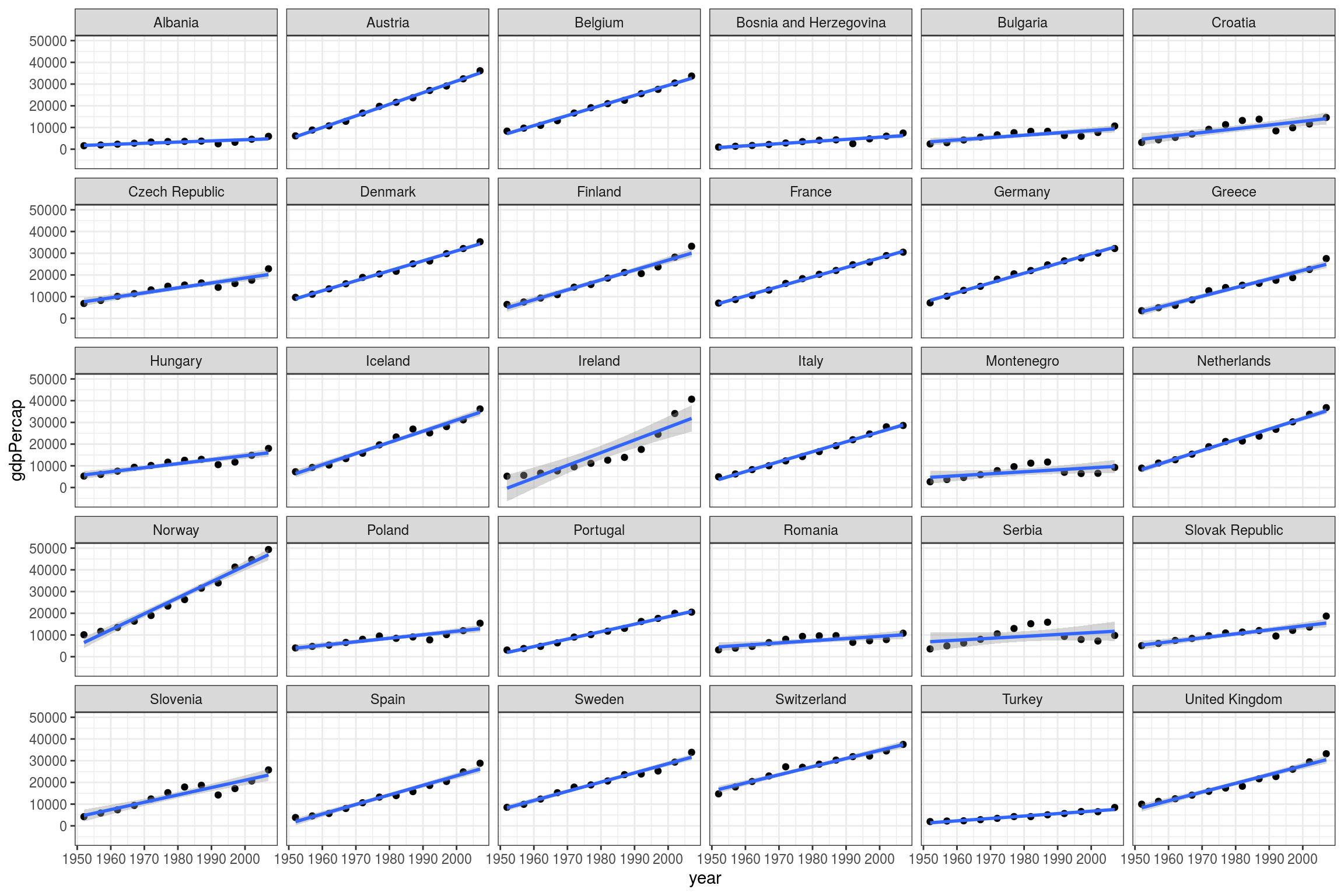

# Countries not linear: Ireland, Montenegro, Serbia.

# Add quadratic term
gapdata %>% 
  filter(continent == "Europe") %>% 
  ggplot(aes(x = year, y = gdpPercap)) + 
  geom_point() +
  geom_smooth(method = "lm", formula = "y ~ poly(x, 2)") +
  facet_wrap(country ~ .)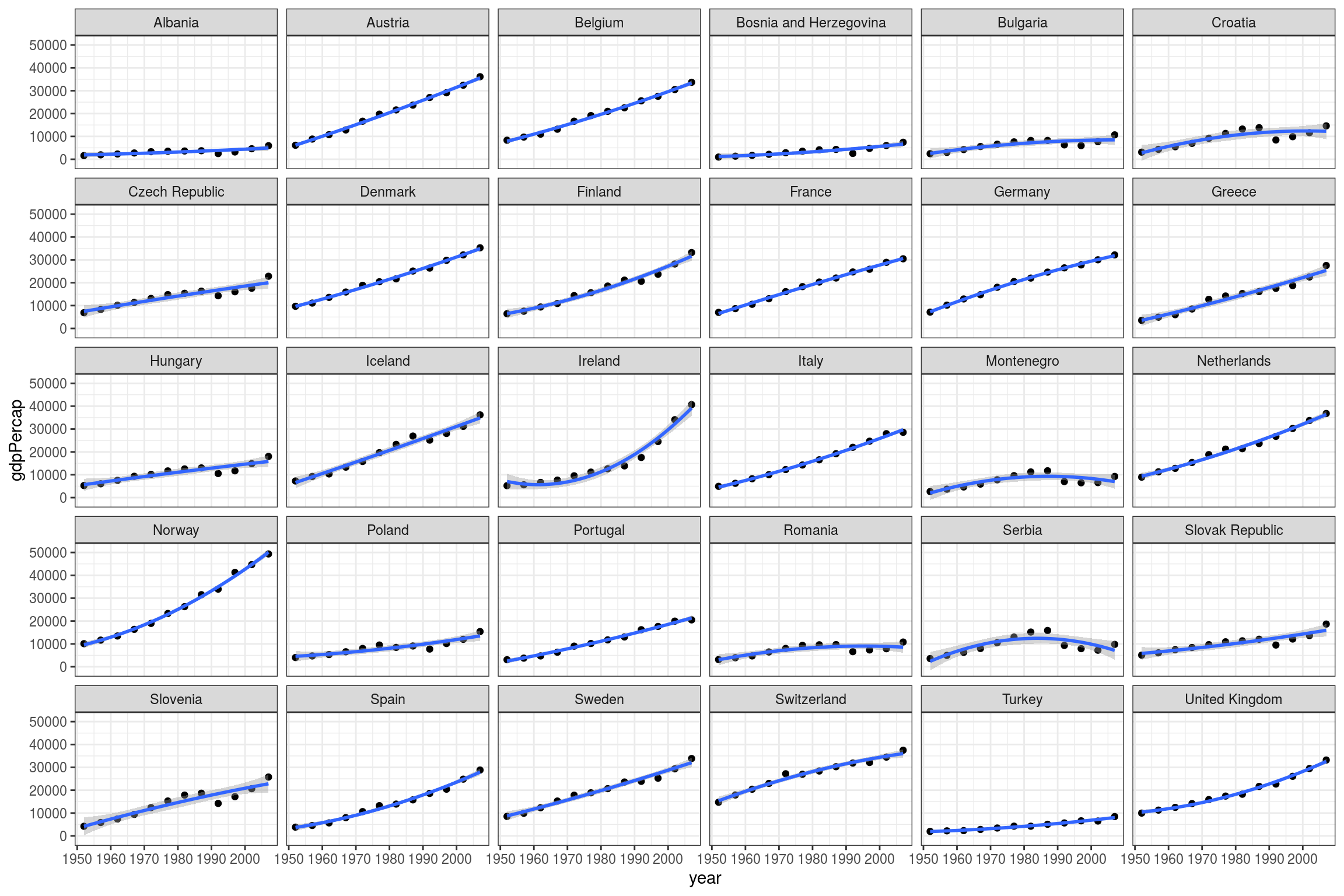

Solution to Exercise 7.4.3:

# Plot first
gapdata %>% 
  filter(country %in% c("Albania", "Austria")) %>% 
  ggplot() + 
  geom_point(aes(x = year, y = gdpPercap, colour= country))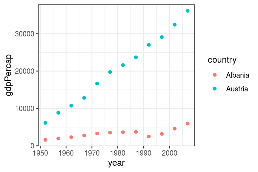

# Fit average line between two countries. 
fit_both1 = gapdata %>% 
  filter(country %in% c("Albania", "Austria")) %>% 
  lm(gdpPercap ~ year, data = .)

gapdata %>% 
  filter(country %in% c("Albania", "Austria")) %>% 
  ggplot() + 
  geom_point(aes(x = year, y = gdpPercap, colour = country)) +
  geom_line(aes(x = year, y = predict(fit_both1)))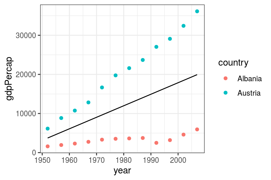

# Fit average line between two countries. 
fit_both3 = gapdata %>% 
  filter(country %in% c("Albania", "Austria")) %>% 
  lm(gdpPercap ~ year * country, data = .)

gapdata %>% 
  filter(country %in% c("Albania", "Austria")) %>% 
  ggplot() + 
  geom_point(aes(x = year, y = gdpPercap, colour = country)) +
  geom_line(aes(x = year, y = predict(fit_both3), group = country))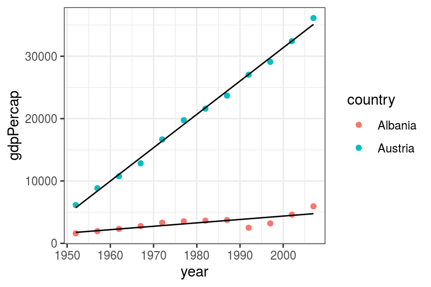

# You can use the regression equation by hand to work out the difference
summary(fit_both3)

# Or pass newdata to predict to estimate the two points of interest
gdp_1980 <- predict(fit_both3, newdata = data.frame(
  country = c("Albania", "Austria"),
  year = c(1980, 1980))
)
gdp_1980
gdp_1980[2] - gdp_1980[1]

Solution to Exercise 7.4.4:

# Plot data first
wcgsdata %>% 
  ggplot(aes(x = age, y = chol))+
  geom_point() + 
  geom_smooth(method = "lm", formula = "y~x")

## Warning: Removed 12 rows containing non-finite values (stat_smooth).

## Warning: Removed 12 rows containing missing values (geom_point).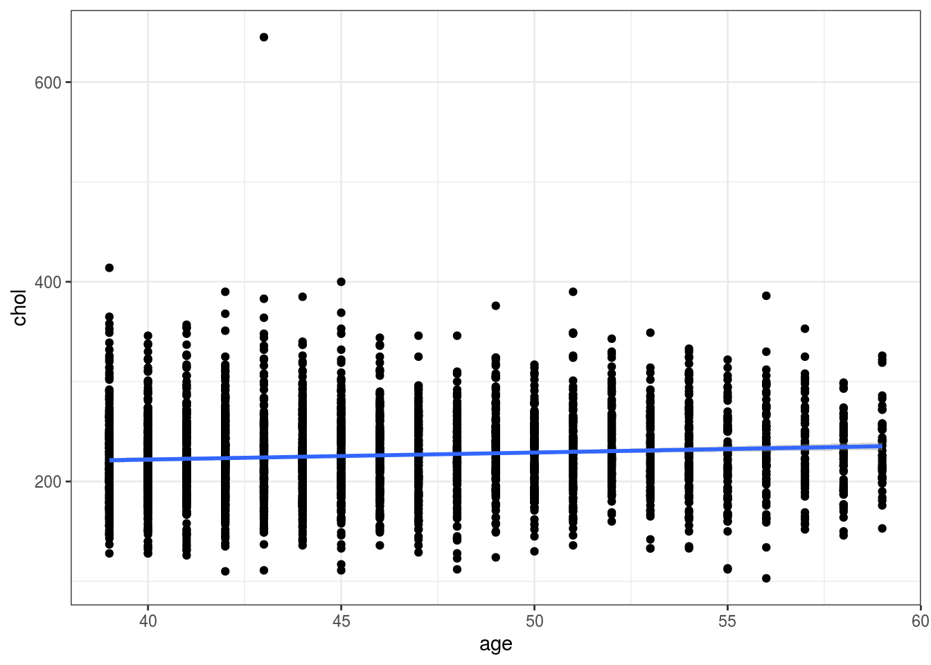

# Weak positive relationship

# Simple linear regression
dependent <- "chol"
explanatory <- "age" 
wcgsdata %>% 
  finalfit(dependent, explanatory, metrics = TRUE)

## Note: dependent includes missing data. These are dropped.

# For each year of age, cholesterol increases by 0.7 mg/100 ml. 
# This gradient differs from zero. 

# Is this effect independent of other available variables?

# Make BMI as above
dependent <- "chol"
explanatory <- c( "age", "bmi", "sbp", "smoking", "personality_2L") 
wcgsdata %>% 
  mutate(
    bmi = ((weight*0.4536) / (height*0.0254)^2) %>% 
      ff_label("BMI")
  ) %>% 
  finalfit(dependent, explanatory, metrics = TRUE)

## Note: dependent includes missing data. These are dropped.

# Effect size is reduced, but still present. 
# Model poorly describes data, R2=0.033.