5.6 Saving your plot
In Chapters 12 and 13 we’ll show you how to export descriptive text, figures, and tables directly from R to Word/PDF/HTML using the power of R Markdown.
The ggsave() function, however, can be used to save a single plot into a variety of formats, namely "pdf" or "png":
If you omit the first argument - the plot object - and call, e.g., ggsave(file = "plot.png) it will just save the last plot that got printed.
Text size tip: playing around with the width and height options (they’re in inches) can be a convenient way to increase or decrease the relative size of the text on the plot.
Look at the relative font sizes of the two versions of the ggsave() call, one 5x4, the other one 10x8 (Figure 5.13):
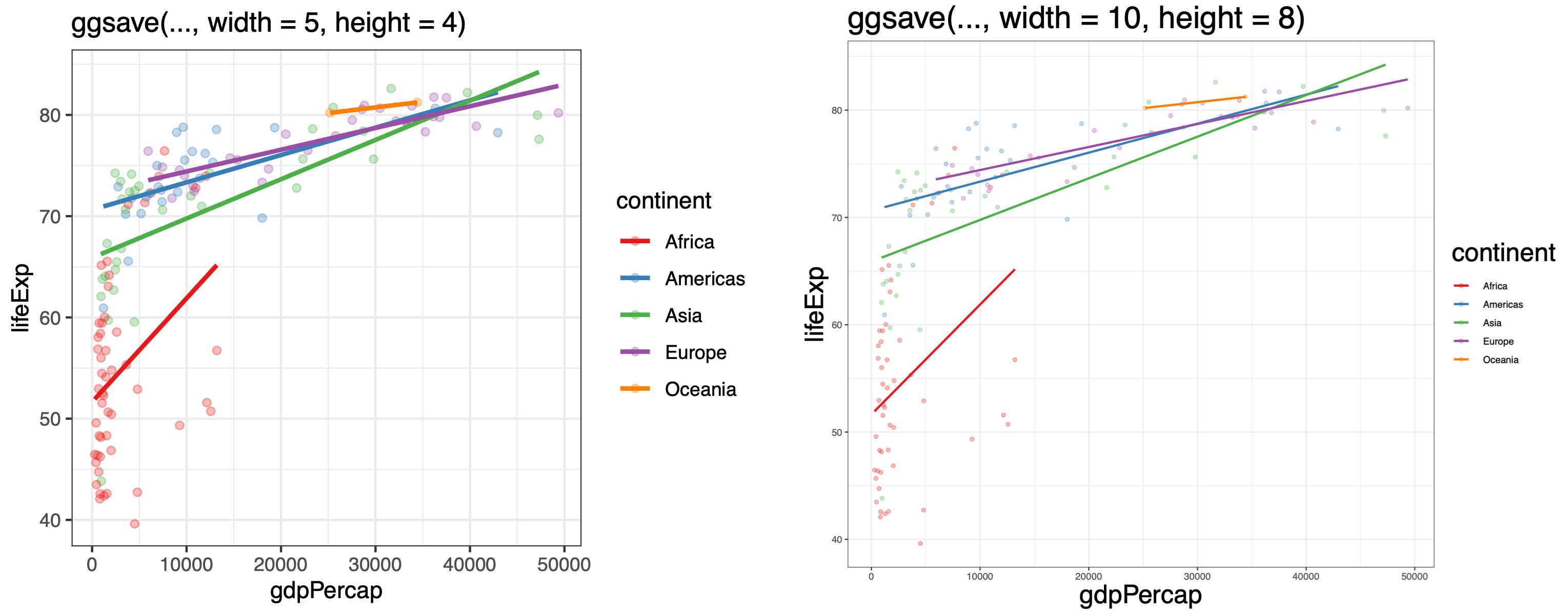
FIGURE 5.13: Experimenting with the width and height options within ggsave() can be used to quickly change how big or small some of the text on your plot looks.
Again, we emphasise the importance of understanding the underlying data through visualisation, rather than relying on statistical tests or, heaven forbid, the p-value alone.
There are five chapters. Testing for continuous outcome variables (6) leads naturally into linear regression (7). We would expect the majority of actual analysis done by readers to be using the methods in chapter 7 rather than 6. Similarly, testing for categorical outcome variables (8) leads naturally to logistic regression (9), where we would expect the majority of work to focus.
Chapters 6 and 8 however do provide helpful reminders of how to prepare data for these analyses and shouldn’t be skipped. time-to-event data (10) introduces survival analysis and includes sections on the manipulation of dates.