9.2 Binary logistic regression
A regression analysis is a statistical approach to estimating the relationships between variables, often by drawing straight lines through data points. For instance, we may try to predict blood pressure in a group of patients based on their coffee consumption (Figure 7.1 from Chapter 7). As blood pressure and coffee consumption can be considered on a continuous scale, this is an example of simple linear regression.
Logistic regression is an extension of this, where the variable being predicted is categorical. We will focus on binary logistic regression, where the dependent variable has two levels, e.g., yes or no, 0 or 1, dead or alive. Other types of logistic regression include ‘ordinal’, when the outcome variable has >2 ordered levels, and ‘multinomial’, where the outcome variable has >2 levels with no inherent order.
We will only deal with binary logistic regression. When we use the term ‘logistic regression’, that is what we are referring to.
We have good reason. In healthcare we are often interested in an event (like death) occurring or not occurring. Binary logistic regression can tell us the probability of this outcome occurring in a patient with a particular set of characteristics.
Although in binary logistic regression the outcome must have two levels, remember that the predictors (explanatory variables) can be either continuous or categorical.
9.2.1 The Question (1)
As in previous chapters, we will use concrete examples when discussing the principles of the approach. We return to our example of coffee drinking. Yes, we are a little obsessed with coffee.
Our outcome variable was previously blood pressure. We will now consider our outcome as the occurrence of a cardiovascular (CV) event over a 10-year period. A cardiovascular event includes the diagnosis of ischemic heart disease, a heart attack (myocardial infarction), or a stroke (cerebrovascular accident). The diagnosis of a cardiovascular event is clearly a binary condition, it either happens or it does not. This is ideal for modelling using binary logistic regression. But remember, the data are completely simulated and not based on anything in the real world. This bit is just for fun!
9.2.2 Odds and probabilities
To understand logistic regression we need to remind ourselves about odds and probability. Odds and probabilities can get confusing so get them straight with Figure 9.1.
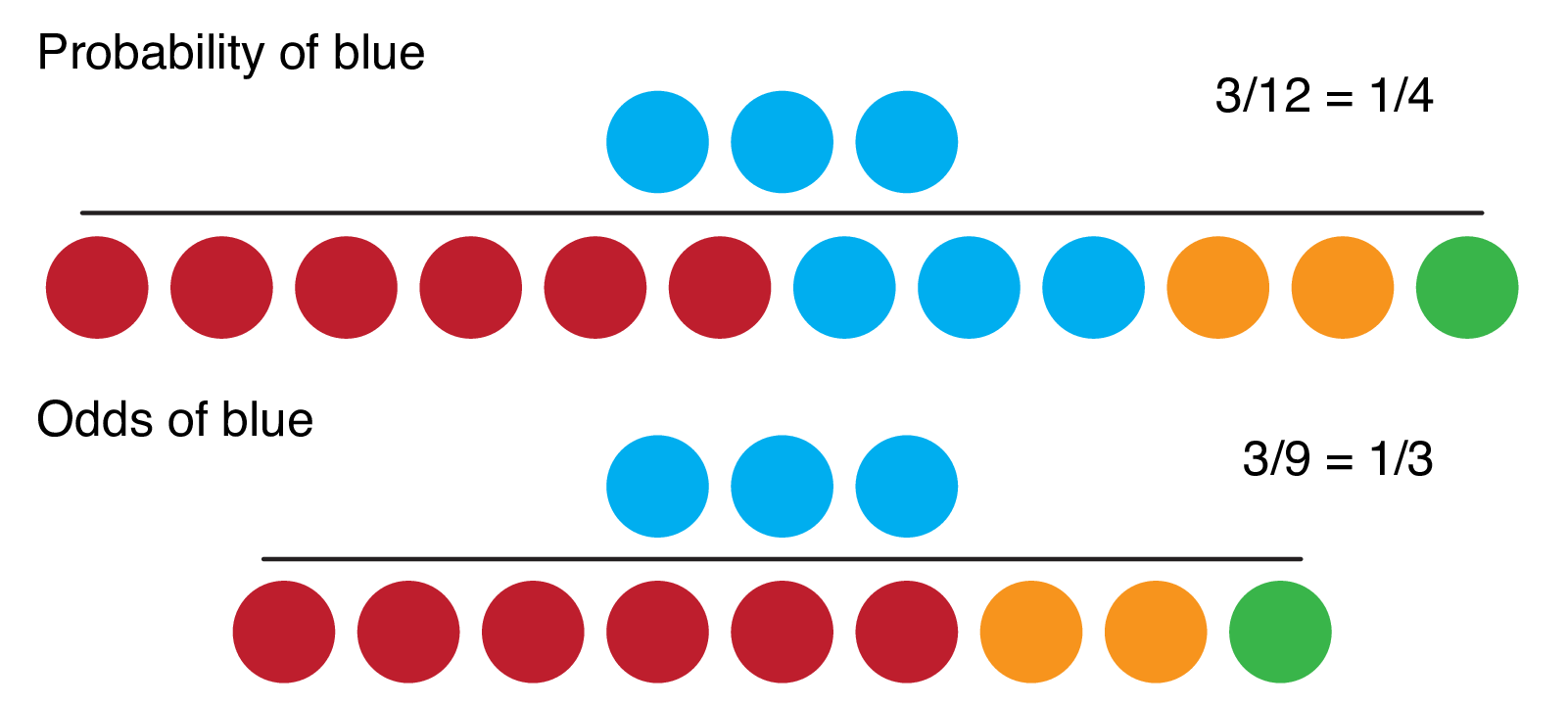
FIGURE 9.1: Probability vs odds.
In many situations, there is no particular reason to prefer one to the other. However, humans seem to have a preference for expressing chance in terms of probabilities, while odds have particular mathematical properties that make them useful in regression.
When a probability is 0, the odds are 0. When a probability is between 0 and 0.5, the odds are less than 1.0 (i.e., less than “1 to 1”). As probability increases from 0.5 to 1.0, the odds increase from 1.0 to approach infinity.
Thus the range of probability is 0 to 1 and the range of odds is 0 to \(+\infty\).
Odds and probabilities can easily be interconverted.
For example, if the odds of a patient dying from a disease are 1/3 (in horse racing this is stated as ‘3 to 1 against’), then the probability of death (also known as risk) is 0.25 (or 25%).
Odds of 1 to 1 equal 50%.
\(Odds = \frac{p}{1-p}\), where \(p\) is the probability of the outcome occurring.
\(Probability = \frac{odds}{odds+1}\).
9.2.3 Odds ratios
Another important term to remind ourselves of is the ‘odds ratio’. Why? Because in a logistic regression the slopes of fitted lines (coefficients) can be interpreted as odds ratios. This is very useful when interpreting the association of a particular predictor with an outcome.
For a given categorical predictor such as smoking, the difference in chance of the outcome occurring for smokers vs non-smokers can be expressed as a ratio of odds or odds ratio (Figure 9.2). For example, if the odds of a smoker having a CV event are 1.5 and the odds of a non-smoker are 1.0, then the odds of a smoker having an event are 1.5-times greater than a non-smoker, odds ratio = 1.5.
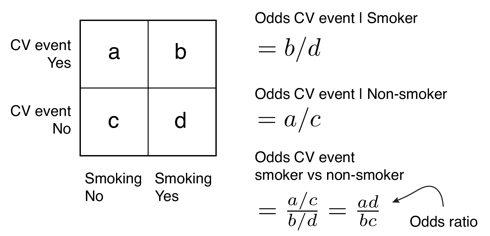
FIGURE 9.2: Odds ratios.
An alternative is a ratio of probabilities which is called a risk ratio or relative risk. We will continue to work with odds ratios given they are an important expression of effect size in logistic regression analysis.
9.2.4 Fitting a regression line
Let’s return to the task at hand. The difficulty in moving from a continuous to a binary outcome variable quickly becomes obvious. If our \(y\)-axis only has two values, say 0 and 1, then how can we fit a line through our data points?
An assumption of linear regression is that the dependent variable is continuous, unbounded, and measured on an interval or ratio scale. Unfortunately, binary dependent variables fulfil none of these requirements.
The answer is what makes logistic regression so useful. Rather than estimating \(y=0\) or \(y=1\) from the \(x\)-axis, we estimate the probability of \(y=1\).
There is one more difficulty in this though. Probabilities can only exist for values of 0 to 1. The probability scale is therefore not linear - straight lines do not make sense on it.
As we saw above, the odds scale runs from 0 to \(+\infty\). But here, probabilities from 0 to 0.5 are squashed into odds of 0 to 1, and probabilities from 0.5 to 1 have the expansive comfort of 1 to \(+\infty\).
This is why we fit binary data on a log-odds scale.
A log-odds scale sounds incredibly off-putting to non-mathematicians, but it is the perfect solution.
- Log-odds run from \(-\infty\) to \(+\infty\);
- odds of 1 become log-odds of 0;
- a doubling and a halving of odds represent the same distance on the scale.
## [1] 0## [1] 0.6931472## [1] -0.6931472I’m sure some are shouting ‘obviously’ at the page. That is good!
This is wrapped up in a transformation (a bit like the transformations shown in Section 6.9.1) using the so-called logit function. This can be skipped with no loss of understanding, but for those who just-gots-to-see, the logit function is,
\(\log_e (\frac{p}{1-p})\), where \(p\) is the probability of the outcome occurring.
Figure 9.3 demonstrates the fitted lines from a logistic regression model of cardiovascular event by coffee consumption, stratified by smoking on the log-odds scale (A) and the probability scale (B). We could conclude, for instance, that on average, non-smokers who drink 2 cups of coffee per day have a 50% chance of a cardiovascular event.
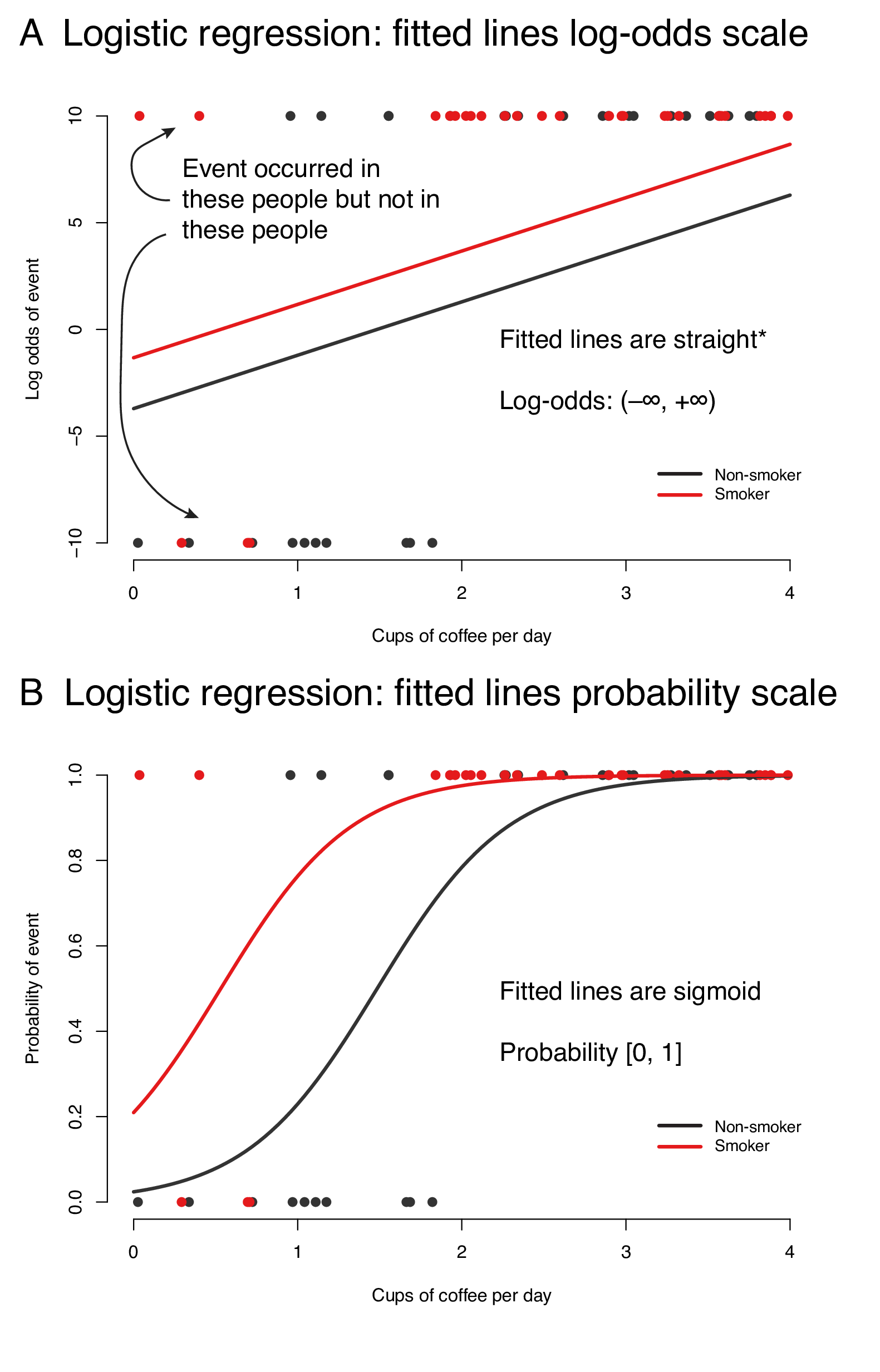
FIGURE 9.3: A logistic regression model of life-time cardiovascular event occurrence by coffee consumption stratified by smoking (simulated data). Fitted lines plotted on the log-odds scale (A) and probability scale (B). *lines are straight when no polynomials or splines are included in regression.
9.2.5 The fitted line and the logistic regression equation
Figure 9.4 links the logistic regression equation, the appearance of the fitted lines on the probability scale, and the output from a standard base R analysis.
The dots at the top and bottom of the plot represent whether individual patients have had an event or not. The fitted line, therefore, represents the point-to-point probability of a patient with a particular set of characteristics having the event or not.
Compare this to Figure 7.4 to be clear on the difference.
The slope of the line is linear on the log-odds scale and these are presented in the output on the log-odds scale.
Thankfully, it is straightforward to convert these to odds ratios, a measure we can use to communicate effect size and direction effectively. Said in more technical language, the exponential of the coefficient on the log-odds scale can be interpreted as an odds ratio.
For a continuous variable such as cups of coffee consumed, the odds ratio is the change in odds of a CV event associated with a 1 cup increase in coffee consumption. We are dealing with linear responses here, so the odds ratio is the same for an increase from 1 to 2 cups, or 3 to 4 cups etc. Remember that if the odds ratio for 1 unit of change is 1.5, then the odds ratio for 2 units of change is \(exp(log(1.5)*2) = 2.25\).
For a categorical variable such as smoking, the odds ratio is the change in odds of a CV event associated with smoking compared with not smoking (the reference level).
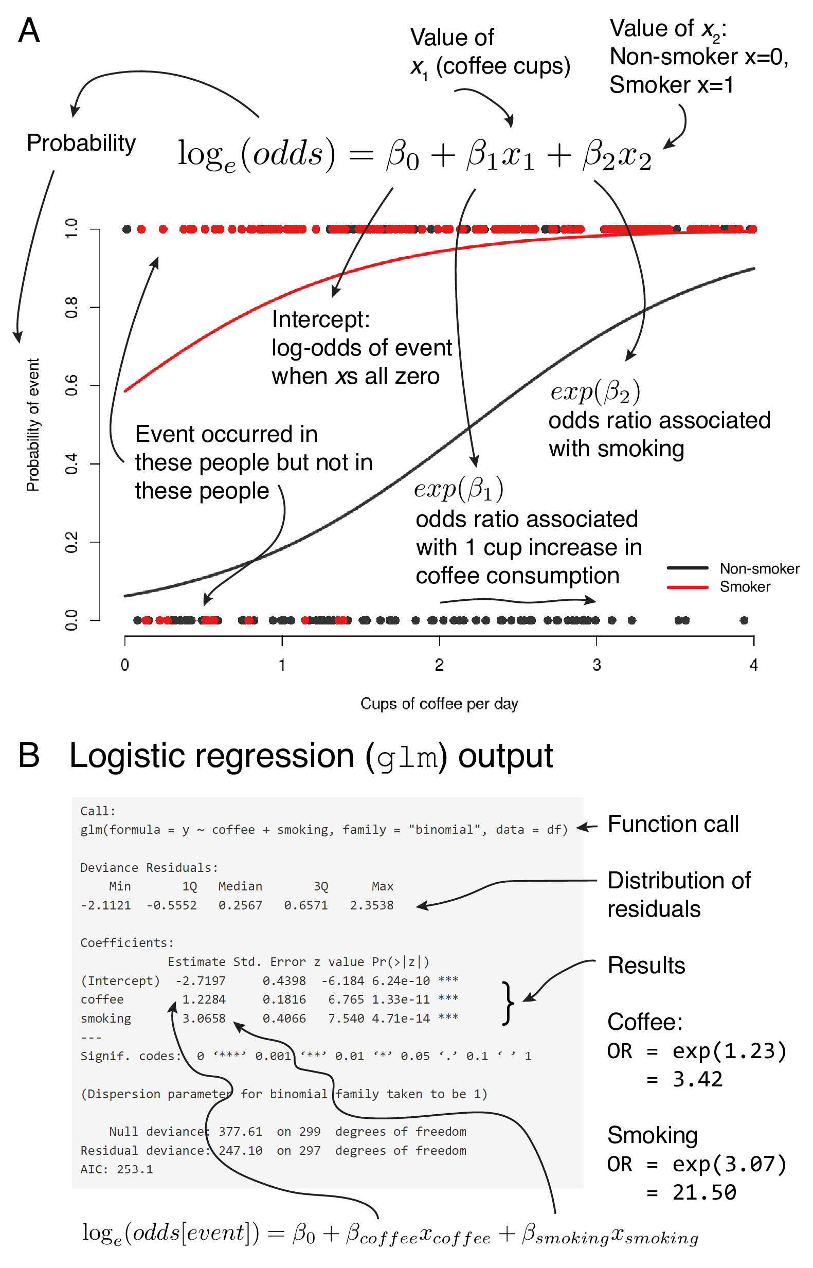
FIGURE 9.4: Linking the logistic regression fitted line and equation (A) with the R output (B).
9.2.6 Effect modification and confounding
As with all multivariable regression models, logistic regression allows the incorporation of multiple variables which all may have direct effects on outcome or may confound the effect of another variable. This was explored in detail in Section 7.1.7; all of the same principles apply.
Adjusting for effect modification and confounding allows us to isolate the direct effect of an explanatory variable of interest upon an outcome. In our example, we are interested in direct effect of coffee drinking on the occurrence of cardiovascular disease, independent of any association between coffee drinking and smoking.
Figure 9.5 demonstrates simple, additive and multiplicative models. Think back to Figure 7.6 and the discussion around it as these terms are easier to think about when looking at the linear regression example, but essentially they work the same way in logistic regression.
Presented on the probability scale, the effect of the interaction is difficult to see. It is obvious on the log-odds scale that the fitted lines are no longer constrained to be parallel.
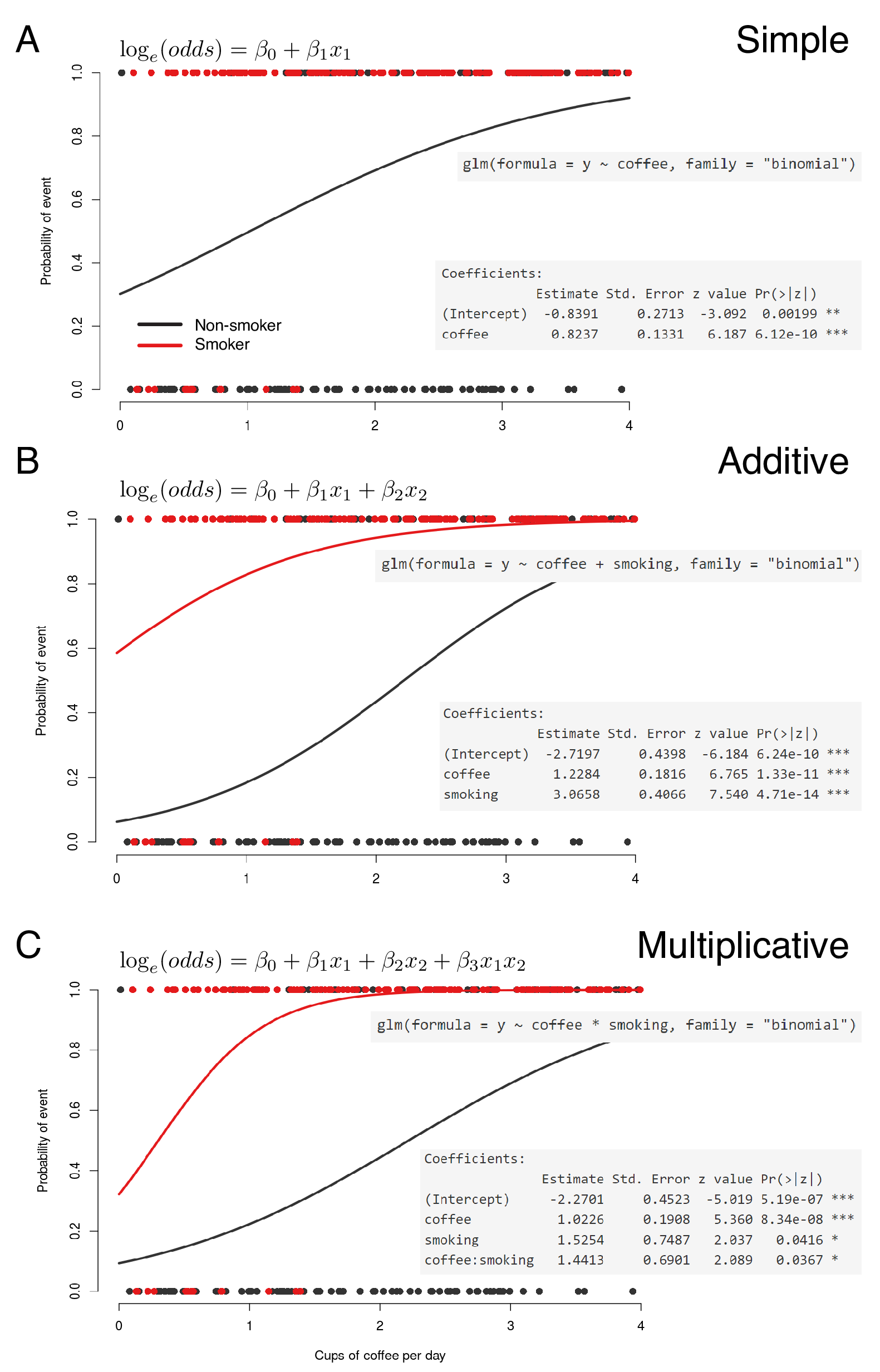
FIGURE 9.5: Multivariable logistic regression (A) with additive (B) and multiplicative (C) effect modification.
The interpretation of the interaction term is important. The exponential of the interaction coefficient term represents a ‘ratio-of-odds ratios’. This is easiest to see through a worked example. In Figure 9.6 the effect of coffee on the odds of a cardiovascular event can be compared in smokers and non-smokers. The effect is now different given the inclusion of a significant interaction term. Please check back to the linear regression chapter if this is not making sense.
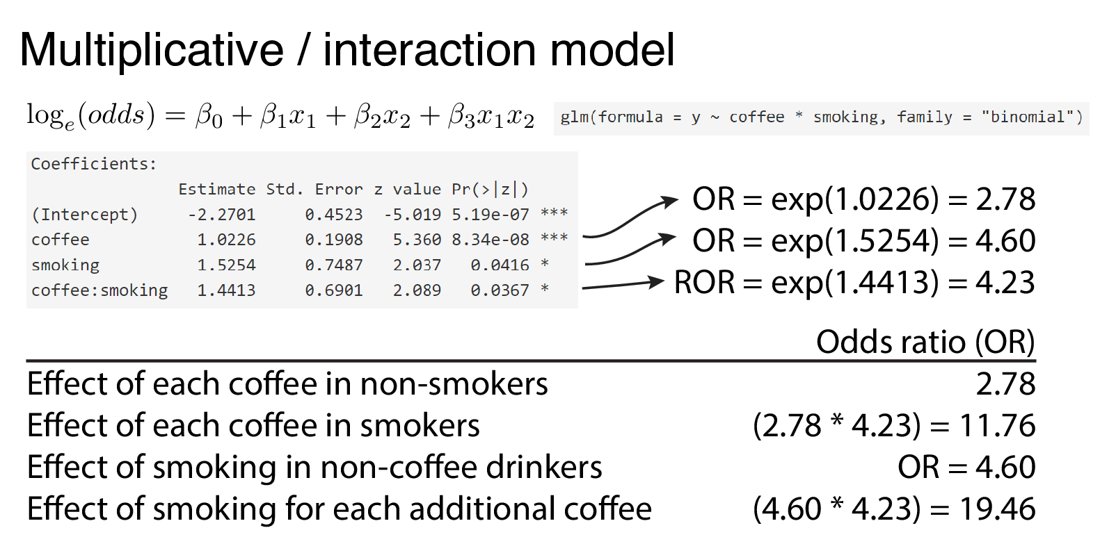
FIGURE 9.6: Multivariable logistic regression with interaction term. The exponential of the interaction term is a ratio-of-odds ratios (ROR).