7.3 Fitting more complex models
7.3.1 The Question (3)
Finally in this section, we are going to fit a more complex linear regression model. Here, we will discuss variable selection and introduce the Akaike Information Criterion (AIC).
We will introduce a new dataset: The Western Collaborative Group Study. This classic dataset includes observations of 3154 healthy young men aged 39-59 from the San Francisco area who were assessed for their personality type. It aimed to capture the occurrence of coronary heart disease over the following 8.5 years.
We will use it, however, to explore the relationship between systolic blood pressure (sbp) and personality type (personality_2L), accounting for potential confounders such as weight (weight).
Now this is just for fun - don’t write in!
The study was designed to look at cardiovascular events as the outcome, not blood pressure. But it is convenient to use blood pressure as a continuous outcome from this dataset, even if that was not the intention of the study.
The included personality types are A: aggressive and B: passive.
7.3.2 Model fitting principles
We suggest building statistical models on the basis of the following six pragmatic principles:
- As few explanatory variables should be used as possible (parsimony);
- Explanatory variables associated with the outcome variable in previous studies should be accounted for;
- Demographic variables should be included in model exploration;
- Population stratification should be incorporated if available;
- Interactions should be checked and included if influential;
- Final model selection should be performed using a “criterion-based approach”
- minimise the Akaike information criterion (AIC)
- maximise the adjusted R-squared value.
This is not the law, but it probably should be. These principles are sensible as we will discuss through the rest of this book. We strongly suggest you do not use automated methods of variable selection. These are often “forward selection” or “backward elimination” methods for including or excluding particular variables on the basis of a statistical property.
In certain settings, these approaches may be found to work. However, they create an artificial distance between you and the problem you are working on. They give you a false sense of certainty that the model you have created is in some sense valid. And quite frequently, they will just get it wrong.
Alternatively, you can follow the six principles above.
A variable may have previously been shown to strongly predict an outcome (think smoking and risk of cancer). This should give you good reason to consider it in your model. But perhaps you think that previous studies were incorrect, or that the variable is confounded by another. All this is fair, but it will be expected that this new knowledge is clearly demonstrated by you, so do not omit these variables before you start.
There are some variables that are so commonly associated with particular outcomes in healthcare that they should almost always be included at the start. Age, sex, social class, and co-morbidity for instance are commonly associated with survival. These need to be assessed before you start looking at your explanatory variable of interest.
Furthermore, patients are often clustered by a particular grouping variable, such as treating hospital. There will be commonalities between these patients that may not be fully explained by your observed variables. To estimate the coefficients of your variables of interest most accurately, clustering should be accounted for in the analysis.
As demonstrated above, the purpose of the model is to provide a best fit approximation of the underlying data. Effect modification and interactions commonly exist in health datasets, and should be incorporated if present.
Finally, we want to assess how well our models fit the data with ‘model checking’.
The effect of adding or removing one variable to the coefficients of the other variables in the model is very important, and will be discussed later.
Measures of goodness-of-fit such as the AIC, can also be of great use when deciding which model choice is most valid.
7.3.3 AIC
The Akaike Information Criterion (AIC) is an alternative goodness-of-fit measure. In that sense, it is similar to the R-squared, but it has a different statistical basis. It is useful because it can be used to help guide the best fit in generalised linear models such as logistic regression (see Chapter 9). It is based on the likelihood but is also penalised for the number of variables present in the model. We aim to have as small an AIC as possible. The value of the number itself has no inherent meaning, but it is used to compare different models of the same data.
7.3.5 Check the data
As always, when you receive a new dataset, carefully check that it does not contain errors.
| label | var_type | n | missing_n | mean | sd | median |
|---|---|---|---|---|---|---|
| Subject ID | <int> | 3154 | 0 | 10477.9 | 5877.4 | 11405.5 |
| Age (years) | <int> | 3154 | 0 | 46.3 | 5.5 | 45.0 |
| Height (inches) | <int> | 3154 | 0 | 69.8 | 2.5 | 70.0 |
| Weight (pounds) | <int> | 3154 | 0 | 170.0 | 21.1 | 170.0 |
| Systolic BP (mmHg) | <int> | 3154 | 0 | 128.6 | 15.1 | 126.0 |
| Diastolic BP (mmHg) | <int> | 3154 | 0 | 82.0 | 9.7 | 80.0 |
| Cholesterol (mg/100 ml) | <int> | 3142 | 12 | 226.4 | 43.4 | 223.0 |
| Cigarettes/day | <int> | 3154 | 0 | 11.6 | 14.5 | 0.0 |
| Time to CHD event | <int> | 3154 | 0 | 2683.9 | 666.5 | 2942.0 |
| label | var_type | n | missing_n | levels_n | levels | levels_count |
|---|---|---|---|---|---|---|
| Personality type | <fct> | 3154 | 0 | 4 |
A1"A2" B3"B4"
|
264, 1325, 1216, 349 |
| Personality type | <fct> | 3154 | 0 | 2 |
B"A"
|
1565, 1589 |
| Smoking | <fct> | 3154 | 0 | 2 |
Non-smoker"Smoker"
|
1652, 1502 |
| Corneal arcus | <fct> | 3152 | 2 | 2 |
No"Yes" (Missing)" </td> <td style="text-align:right;width: 3cm; "> 2211, 941, 2 </td> </tr> <tr> <td style="text-align:left;"> CHD event </td> <td style="text-align:left;"> <fct> </td> <td style="text-align:right;"> 3154 </td> <td style="text-align:right;"> 0 </td> <td style="text-align:right;"> 2 </td> <td style="text-align:right;width: 3cm; ">No" Yes" </td> <td style="text-align:right;width: 3cm; "> 2897, 257 </td> </tr> <tr> <td style="text-align:left;"> Type CHD </td> <td style="text-align:left;"> <fct> </td> <td style="text-align:right;"> 3154 </td> <td style="text-align:right;"> 0 </td> <td style="text-align:right;"> 4 </td> <td style="text-align:right;width: 3cm; ">No" MI_SD"Silent_MI" ``Angina"
|
2897, 135, 71, 51 |
7.3.6 Plot the data
wcgsdata %>%
  ggplot(aes(y = sbp, x = weight,
             colour = personality_2L)) +   # Personality type
  geom_point(alpha = 0.2) +                # Add transparency
  geom_smooth(method = "lm", se = FALSE)
## `geom_smooth()` using formula 'y ~ x'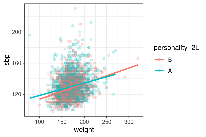
FIGURE 7.12: Scatter and line plot. Systolic blood pressure by weight and personality type.
From Figure 7.12, we can see that there is a weak relationship between weight and blood pressure.
In addition, there is really no meaningful effect of personality type on blood pressure. This is really important because, as you will see below, we are about to “find” some highly statistically significant effects in a model.
7.3.7 Linear regression with finalfit
finalfit is our own package and provides a convenient set of functions for fitting regression models with results presented in final tables.
There are a host of features with example code at the finalfit website.
Here we will use the all-in-one finalfit() function, which takes a dependent variable and one or more explanatory variables.
The appropriate regression for the dependent variable is performed, from a choice of linear, logistic, and Cox Proportional Hazards regression models.
Summary statistics, together with a univariable and a multivariable regression analysis are produced in a final results table.
dependent <- "sbp"
explanatory <- "personality_2L"
fit_sbp1 <- wcgsdata %>%
finalfit(dependent, explanatory, metrics = TRUE)| Dependent: Systolic BP (mmHg) | unit | value | Coefficient (univariable) | Coefficient (multivariable) | |
|---|---|---|---|---|---|
| Personality type | B | Mean (sd) | 127.5 (14.4) |
|
|
| A | Mean (sd) | 129.8 (15.7) | 2.32 (1.26 to 3.37, p<0.001) | 2.32 (1.26 to 3.37, p<0.001) |
| Number in dataframe = 3154, Number in model = 3154, Missing = 0, Log-likelihood = -13031.39, AIC = 26068.8, R-squared = 0.0059, Adjusted R-squared = 0.0056 |
Let’s look first at our explanatory variable of interest, personality type. When a factor is entered into a regression model, the default is to compare each level of the factor with a “reference level”. What you choose as the reference level can be easily changed (see Section 8.9. Alternative methods are available (sometimes called contrasts), but the default method is likely to be what you want almost all the time. Note this is sometimes referred to as creating a “dummy variable”.
It can be seen that the mean blood pressure for type A is higher than for type B.
As there is only one variable, the univariable and multivariable analyses are the same (the multivariable column can be removed if desired by including select(-5) #5th column in the piped function).
Although the difference is numerically quite small (2.3 mmHg), it is statistically significant partly because of the large number of patients in the study.
The optional metrics = TRUE output gives us the number of rows (in this case, subjects) included in the model.
This is important as frequently people forget that in standard regression models, missing data from any variable results in the entire row being excluded from the analysis (see Chapter 11).
Note the AIC and Adjusted R-squared results.
The adjusted R-squared is very low - the model only explains only 0.6% of the variation in systolic blood pressure.
This is to be expected, given our scatter plot above.
Let’s now include subject weight, which we have hypothesised may influence blood pressure.
dependent <- "sbp"
explanatory <- c("weight", "personality_2L")
fit_sbp2 <- wcgsdata %>%
finalfit(dependent, explanatory, metrics = TRUE)| Dependent: Systolic BP (mmHg) | unit | value | Coefficient (univariable) | Coefficient (multivariable) | |
|---|---|---|---|---|---|
| Weight (pounds) | [78.0,320.0] | Mean (sd) | 128.6 (15.1) | 0.18 (0.16 to 0.21, p<0.001) | 0.18 (0.16 to 0.20, p<0.001) |
| Personality type | B | Mean (sd) | 127.5 (14.4) |
|
|
| A | Mean (sd) | 129.8 (15.7) | 2.32 (1.26 to 3.37, p<0.001) | 1.99 (0.97 to 3.01, p<0.001) |
| Number in dataframe = 3154, Number in model = 3154, Missing = 0, Log-likelihood = -12928.82, AIC = 25865.6, R-squared = 0.068, Adjusted R-squared = 0.068 |
The output shows us the range for weight (78 to 320 pounds) and the mean (standard deviation) systolic blood pressure for the whole cohort.
The coefficient with 95% confidence interval is provided by default. This is interpreted as: for each pound increase in weight, there is on average a corresponding increase of 0.18 mmHg in systolic blood pressure.
Note the difference in the interpretation of continuous and categorical variables in the regression model output (Table 7.4).
The adjusted R-squared is now higher - the personality and weight together explain 6.8% of the variation in blood pressure.
The AIC is also slightly lower meaning this new model better fits the data.
There is little change in the size of the coefficients for each variable in the multivariable analysis, meaning that they are reasonably independent. As an exercise, check the distribution of weight by personality type using a boxplot.
Let’s now add in other variables that may influence systolic blood pressure.
dependent <- "sbp"
explanatory <- c("personality_2L", "weight", "age",
                "height", "chol", "smoking")
fit_sbp3 <- wcgsdata %>%
finalfit(dependent, explanatory, metrics = TRUE)| Dependent: Systolic BP (mmHg) | unit | value | Coefficient (univariable) | Coefficient (multivariable) | |
|---|---|---|---|---|---|
| Personality type | B | Mean (sd) | 127.5 (14.4) |
|
|
| A | Mean (sd) | 129.8 (15.7) | 2.32 (1.26 to 3.37, p<0.001) | 1.44 (0.44 to 2.43, p=0.005) | |
| Weight (pounds) | [78.0,320.0] | Mean (sd) | 128.6 (15.1) | 0.18 (0.16 to 0.21, p<0.001) | 0.24 (0.21 to 0.27, p<0.001) |
| Age (years) | [39.0,59.0] | Mean (sd) | 128.6 (15.1) | 0.45 (0.36 to 0.55, p<0.001) | 0.43 (0.33 to 0.52, p<0.001) |
| Height (inches) | [60.0,78.0] | Mean (sd) | 128.6 (15.1) | 0.11 (-0.10 to 0.32, p=0.302) | -0.84 (-1.08 to -0.61, p<0.001) |
| Cholesterol (mg/100 ml) | [103.0,645.0] | Mean (sd) | 128.6 (15.1) | 0.04 (0.03 to 0.05, p<0.001) | 0.03 (0.02 to 0.04, p<0.001) |
| Smoking | Non-smoker | Mean (sd) | 128.6 (15.6) |
|
|
| Smoker | Mean (sd) | 128.7 (14.6) | 0.08 (-0.98 to 1.14, p=0.883) | 0.95 (-0.05 to 1.96, p=0.063) |
| Number in dataframe = 3154, Number in model = 3142, Missing = 12, Log-likelihood = -12772.04, AIC = 25560.1, R-squared = 0.12, Adjusted R-squared = 0.12 |
Age, height, serum cholesterol, and smoking status have been added. Some of the variation explained by personality type has been taken up by these new variables - personality is now associated with an average change of blood pressure of 1.4 mmHg.
The adjusted R-squared now tells us that 12% of the variation in blood pressure is explained by the model, which is an improvement.
Look out for variables that show large changes in effect size or a change in the direction of effect when going from a univariable to multivariable model. This means that the other variables in the model are having a large effect on this variable and the cause of this should be explored. For instance, in this example the effect of height changes size and direction. This is because of the close association between weight and height. For instance, it may be more sensible to work with body mass index (\(weight / height^2\)) rather than the two separate variables.
In general, variables that are highly correlated with each other should be treated carefully in regression analysis. This is called collinearity and can lead to unstable estimates of coefficients. For more on this, see Section 9.4.2.
Let’s create a new variable called bmi, note the conversion from pounds and inches to kg and m:
Weight and height can now be replaced in the model with BMI.
explanatory <- c("personality_2L", "bmi", "age",
                "chol", "smoking")

fit_sbp4 <- wcgsdata %>%
finalfit(dependent, explanatory, metrics = TRUE)| Dependent: Systolic BP (mmHg) | unit | value | Coefficient (univariable) | Coefficient (multivariable) | |
|---|---|---|---|---|---|
| Personality type | B | Mean (sd) | 127.5 (14.4) |
|
|
| A | Mean (sd) | 129.8 (15.7) | 2.32 (1.26 to 3.37, p<0.001) | 1.51 (0.51 to 2.50, p=0.003) | |
| BMI | [11.2,39.0] | Mean (sd) | 128.6 (15.1) | 1.69 (1.50 to 1.89, p<0.001) | 1.65 (1.46 to 1.85, p<0.001) |
| Age (years) | [39.0,59.0] | Mean (sd) | 128.6 (15.1) | 0.45 (0.36 to 0.55, p<0.001) | 0.41 (0.32 to 0.50, p<0.001) |
| Cholesterol (mg/100 ml) | [103.0,645.0] | Mean (sd) | 128.6 (15.1) | 0.04 (0.03 to 0.05, p<0.001) | 0.03 (0.02 to 0.04, p<0.001) |
| Smoking | Non-smoker | Mean (sd) | 128.6 (15.6) |
|
|
| Smoker | Mean (sd) | 128.7 (14.6) | 0.08 (-0.98 to 1.14, p=0.883) | 0.98 (-0.03 to 1.98, p=0.057) |
| Number in dataframe = 3154, Number in model = 3142, Missing = 12, Log-likelihood = -12775.03, AIC = 25564.1, R-squared = 0.12, Adjusted R-squared = 0.12 |
On the principle of parsimony, we may want to remove variables which are not contributing much to the model.
For instance, let’s compare models with and without the inclusion of smoking.
This can be easily done using the finalfit explanatory_multi option.
dependent <- "sbp"
explanatory       <- c("personality_2L", "bmi", "age",
                      "chol", "smoking")
explanatory_multi <- c("bmi", "personality_2L", "age",
                      "chol")
fit_sbp5 <- wcgsdata %>%
  finalfit(dependent, explanatory,
           explanatory_multi,
keep_models = TRUE, metrics = TRUE)| Dependent: Systolic BP (mmHg) | unit | value | Coefficient (univariable) | Coefficient (multivariable) | Coefficient (multivariable reduced) | |
|---|---|---|---|---|---|---|
| Personality type | B | Mean (sd) | 127.5 (14.4) |
|
|
|
| A | Mean (sd) | 129.8 (15.7) | 2.32 (1.26 to 3.37, p<0.001) | 1.51 (0.51 to 2.50, p=0.003) | 1.56 (0.57 to 2.56, p=0.002) | |
| BMI | [11.2,39.0] | Mean (sd) | 128.6 (15.1) | 1.69 (1.50 to 1.89, p<0.001) | 1.65 (1.46 to 1.85, p<0.001) | 1.62 (1.43 to 1.82, p<0.001) |
| Age (years) | [39.0,59.0] | Mean (sd) | 128.6 (15.1) | 0.45 (0.36 to 0.55, p<0.001) | 0.41 (0.32 to 0.50, p<0.001) | 0.41 (0.32 to 0.50, p<0.001) |
| Cholesterol (mg/100 ml) | [103.0,645.0] | Mean (sd) | 128.6 (15.1) | 0.04 (0.03 to 0.05, p<0.001) | 0.03 (0.02 to 0.04, p<0.001) | 0.03 (0.02 to 0.04, p<0.001) |
| Smoking | Non-smoker | Mean (sd) | 128.6 (15.6) |
|
|
|
| Smoker | Mean (sd) | 128.7 (14.6) | 0.08 (-0.98 to 1.14, p=0.883) | 0.98 (-0.03 to 1.98, p=0.057) |
|
| Number in dataframe = 3154, Number in model = 3142, Missing = 12, Log-likelihood = -12775.03, AIC = 25564.1, R-squared = 0.12, Adjusted R-squared = 0.12 |
| Number in dataframe = 3154, Number in model = 3142, Missing = 12, Log-likelihood = -12776.83, AIC = 25565.7, R-squared = 0.12, Adjusted R-squared = 0.12 |
This results in little change in the other coefficients and very little change in the AIC. We will consider the reduced model the final model.
We can also visualise models using plotting. This is useful for communicating a model in a restricted space, e.g., in a presentation.
dependent <- "sbp"
explanatory       <- c("personality_2L", "bmi", "age",
                      "chol", "smoking")
explanatory_multi <- c("bmi", "personality_2L", "age",
                      "chol")
fit_sbp5 <- wcgsdata %>%
  ff_plot(dependent, explanatory_multi)
We can check the assumptions as above.
dependent <- "sbp"
explanatory_multi <- c("bmi", "personality_2L", "age",
                      "chol")
wcgsdata %>%
  lmmulti(dependent, explanatory_multi) %>%
  autoplot()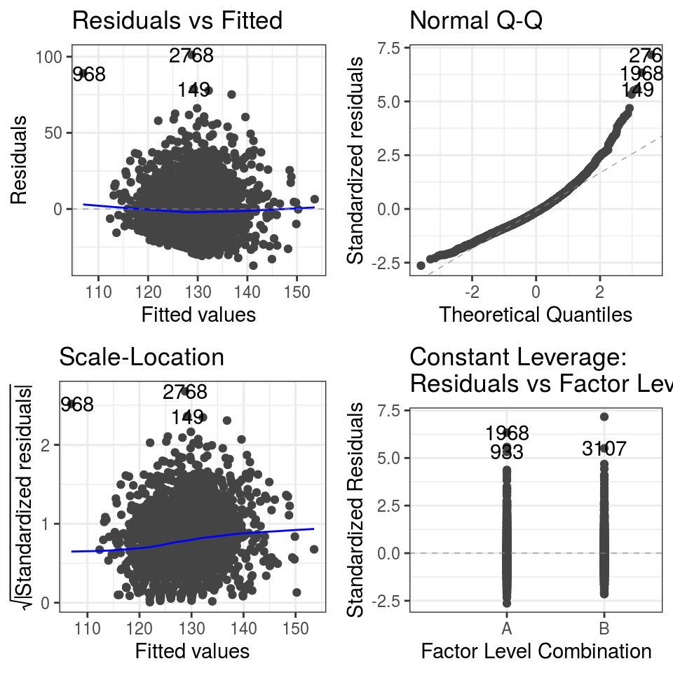
FIGURE 7.13: Diagnostic plots: Linear regression model of systolic blood pressure.
An important message in the results relates to the highly significant p-values in the table above. Should we conclude that in a multivariable regression model controlling for BMI, age, and serum cholesterol, blood pressure was significantly elevated in those with a Type A personality (1.56 (0.57 to 2.56, p=0.002) compared with Type B? The p-value looks impressive, but the actual difference in blood pressure is only 1.6 mmHg. Even at a population level, that may not be clinically significant, fitting with our first thoughts when we saw the scatter plot.
This serves to emphasise our most important point. Our focus should be on understanding the underlying data itself, rather than relying on complex multidimensional modelling procedures. By making liberal use of upfront plotting, together with further visualisation as you understand the data, you will likely be able to draw most of the important conclusions that the data has to offer. Use modelling to quantify and confirm this, rather than as the primary method of data exploration.
7.3.8 Summary
Time spent truly understanding linear regression is well spent. Not because you will spend a lot of time making linear regression models in health data science (we rarely do), but because it the essential foundation for understanding more advanced statistical models.
It can even be argued that all common statistical tests are linear models. This great post demonstrates beautifully how the statistical tests we are most familiar with (such as t-test, Mann-Whitney U test, ANOVA, chi-squared test) can simply be considered as special cases of linear models, or close approximations.
Regression is fitting lines, preferably straight, through data points. Make \(\hat{y} = \beta_0 + \beta_1 x_1\) a close friend.
An excellent book for further reading on regression is Harrell (2015).
References
Harrell, Frank. 2015. Regression Modeling Strategies: With Applications to Linear Models, Logistic and Ordinal Regression, and Survival Analysis. 2nd ed. Springer Series in Statistics. Springer International Publishing. https://doi.org/10.1007/978-3-319-19425-7.