9.8 Model fitting
Engage with the data and the results when model fitting. Do not use automated processes - you have to keep thinking.
Three things are important to keep looking at:
- what is the association between a particular variable and the outcome (OR and 95%CI);
- how much information is a variable bringing to the model (change in AIC and c-statistic);
- how much influence does adding a variable have on the effect size of another variable, and in particular my variable of interest (a rule of thumb is seeing a greater than 10% change in the OR of the variable of interest when a new variable is added to the model, suggests the new variable is important).
We’re going to start by including the variables from above which we think are relevant.
library(finalfit)
dependent <- "mort_5yr"
explanatory <- c("ulcer.factor", "age", "sex.factor", "t_stage.factor")
fit2 = melanoma %>%
finalfit(dependent, explanatory, metrics = TRUE)| Dependent: 5-year survival | No | Yes | OR (univariable) | OR (multivariable) | |
|---|---|---|---|---|---|
| Ulcerated tumour | Absent | 105 (91.3) | 10 (8.7) |
|
|
| Present | 55 (61.1) | 35 (38.9) | 6.68 (3.18-15.18, p<0.001) | 3.21 (1.32-8.28, p=0.012) | |
| Age (years) | Mean (SD) | 51.7 (16.0) | 55.3 (18.8) | 1.01 (0.99-1.03, p=0.202) | 1.00 (0.98-1.02, p=0.948) |
| Sex | Female | 105 (83.3) | 21 (16.7) |
|
|
| Male | 55 (69.6) | 24 (30.4) | 2.18 (1.12-4.30, p=0.023) | 1.26 (0.57-2.76, p=0.558) | |
| T-stage | T1 | 52 (92.9) | 4 (7.1) |
|
|
| T2 | 49 (92.5) | 4 (7.5) | 1.06 (0.24-4.71, p=0.936) | 0.77 (0.16-3.58, p=0.733) | |
| T3 | 36 (70.6) | 15 (29.4) | 5.42 (1.80-20.22, p=0.005) | 2.98 (0.86-12.10, p=0.098) | |
| T4 | 23 (51.1) | 22 (48.9) | 12.43 (4.21-46.26, p<0.001) | 4.98 (1.34-21.64, p=0.021) |
| Number in dataframe = 205, Number in model = 205, Missing = 0, AIC = 188.1, C-statistic = 0.798, H&L = Chi-sq(8) 3.92 (p=0.864) |
The model metrics have improved with the AIC decreasing from 192 to 188 and the c-statistic increasing from 0.717 to 0.798.
Let’s consider age.
We may expect age to be associated with the outcome because it so commonly is.
But there is weak evidence of an association in the univariable analysis.
We have shown above that the relationship of age to the outcome is not linear, therefore we need to act on this.
We can either convert age to a categorical variable or include it with a quadratic term (\(x^2 + x\), remember parabolas from school?).
melanoma <- melanoma %>%
  mutate(
    age.factor = cut(age,
                     breaks = c(0, 25, 50, 75, 100)) %>%
      ff_label("Age (years)"))

# Add this to relevel:
# fct_relevel("(50,75]")

melanoma %>%
finalfit(dependent, c("ulcer.factor", "age.factor"), metrics = TRUE)| Dependent: 5-year survival | No | Yes | OR (univariable) | OR (multivariable) | |
|---|---|---|---|---|---|
| Ulcerated tumour | Absent | 105 (91.3) | 10 (8.7) |
|
|
| Present | 55 (61.1) | 35 (38.9) | 6.68 (3.18-15.18, p<0.001) | 6.28 (2.97-14.35, p<0.001) | |
| Age (years) | (0,25] | 10 (71.4) | 4 (28.6) |
|
|
| (25,50] | 62 (84.9) | 11 (15.1) | 0.44 (0.12-1.84, p=0.229) | 0.54 (0.13-2.44, p=0.400) | |
| (50,75] | 79 (76.0) | 25 (24.0) | 0.79 (0.24-3.08, p=0.712) | 0.81 (0.22-3.39, p=0.753) | |
| (75,100] | 9 (64.3) | 5 (35.7) | 1.39 (0.28-7.23, p=0.686) | 1.12 (0.20-6.53, p=0.894) |
| Number in dataframe = 205, Number in model = 205, Missing = 0, AIC = 196.6, C-statistic = 0.742, H&L = Chi-sq(8) 0.20 (p=1.000) |
There is no strong relationship between the categorical representation of age and the outcome. Let’s try a quadratic term.
In base R, a quadratic term is added like this.
##
## Call:
## glm(formula = mort_5yr ~ ulcer.factor + I(age^2) + age, family = binomial,
##     data = melanoma)
##
## Deviance Residuals:
##     Min       1Q   Median       3Q      Max
## -1.3253  -0.8973  -0.4082  -0.3889   2.2872
##
## Coefficients:
##                       Estimate Std. Error z value Pr(>|z|)
## (Intercept)         -1.2636638  1.2058471  -1.048    0.295
## ulcer.factorPresent  1.8423431  0.3991559   4.616 3.92e-06 ***
## I(age^2)             0.0006277  0.0004613   1.361    0.174
## age                 -0.0567465  0.0476011  -1.192    0.233
## ---
## Signif. codes:  0 '***' 0.001 '**' 0.01 '*' 0.05 '.' 0.1 ' ' 1
##
## (Dispersion parameter for binomial family taken to be 1)
##
##     Null deviance: 215.78  on 204  degrees of freedom
## Residual deviance: 185.98  on 201  degrees of freedom
## AIC: 193.98
##
## Number of Fisher Scoring iterations: 5
It can be done in Finalfit in a similar manner.
Note with default univariable model settings, the quadratic and linear terms are considered in separate models, which doesn’t make much sense.
library(finalfit)
dependent <- "mort_5yr"
explanatory <- c("ulcer.factor", "I(age^2)", "age")
melanoma %>%
finalfit(dependent, explanatory, metrics = TRUE)| Dependent: 5-year survival | No | Yes | OR (univariable) | OR (multivariable) | |
|---|---|---|---|---|---|
| Ulcerated tumour | Absent | 105 (91.3) | 10 (8.7) |
|
|
| Present | 55 (61.1) | 35 (38.9) | 6.68 (3.18-15.18, p<0.001) | 6.31 (2.98-14.44, p<0.001) | |
| Age (years) | Mean (SD) | 51.7 (16.0) | 55.3 (18.8) | 1.01 (0.99-1.03, p=0.202) | 0.94 (0.86-1.04, p=0.233) |
| I(age^2) | 1.00 (1.00-1.00, p=0.101) | 1.00 (1.00-1.00, p=0.174) |
| Number in dataframe = 205, Number in model = 205, Missing = 0, AIC = 194, C-statistic = 0.748, H&L = Chi-sq(8) 5.24 (p=0.732) |
The AIC is worse when adding age either as a factor or with a quadratic term to the base model.
One final method to visualise the contribution of a particular variable is to remove it from the full model.
This is convenient in Finalfit.
library(finalfit)
dependent <- "mort_5yr"
explanatory <- c("ulcer.factor", "age.factor", "sex.factor", "t_stage.factor")
explanatory_multi <- c("ulcer.factor", "sex.factor", "t_stage.factor")

melanoma %>%
  finalfit(dependent, explanatory, explanatory_multi,
keep_models = TRUE, metrics = TRUE)| Dependent: 5-year survival | No | Yes | OR (univariable) | OR (multivariable) | OR (multivariable reduced) | |
|---|---|---|---|---|---|---|
| Ulcerated tumour | Absent | 105 (91.3) | 10 (8.7) |
|
|
|
| Present | 55 (61.1) | 35 (38.9) | 6.68 (3.18-15.18, p<0.001) | 3.06 (1.25-7.93, p=0.017) | 3.21 (1.32-8.28, p=0.012) | |
| Age (years) | (0,25] | 10 (71.4) | 4 (28.6) |
|
|
|
| (25,50] | 62 (84.9) | 11 (15.1) | 0.44 (0.12-1.84, p=0.229) | 0.37 (0.08-1.80, p=0.197) |
|
|
| (50,75] | 79 (76.0) | 25 (24.0) | 0.79 (0.24-3.08, p=0.712) | 0.60 (0.15-2.65, p=0.469) |
|
|
| (75,100] | 9 (64.3) | 5 (35.7) | 1.39 (0.28-7.23, p=0.686) | 0.61 (0.09-4.04, p=0.599) |
|
|
| Sex | Female | 105 (83.3) | 21 (16.7) |
|
|
|
| Male | 55 (69.6) | 24 (30.4) | 2.18 (1.12-4.30, p=0.023) | 1.21 (0.54-2.68, p=0.633) | 1.26 (0.57-2.76, p=0.559) | |
| T-stage | T1 | 52 (92.9) | 4 (7.1) |
|
|
|
| T2 | 49 (92.5) | 4 (7.5) | 1.06 (0.24-4.71, p=0.936) | 0.74 (0.15-3.50, p=0.697) | 0.77 (0.16-3.58, p=0.733) | |
| T3 | 36 (70.6) | 15 (29.4) | 5.42 (1.80-20.22, p=0.005) | 2.91 (0.84-11.82, p=0.106) | 2.99 (0.86-12.11, p=0.097) | |
| T4 | 23 (51.1) | 22 (48.9) | 12.43 (4.21-46.26, p<0.001) | 5.38 (1.43-23.52, p=0.016) | 5.01 (1.37-21.52, p=0.020) |
| Number in dataframe = 205, Number in model = 205, Missing = 0, AIC = 190, C-statistic = 0.802, H&L = Chi-sq(8) 13.87 (p=0.085) |
| Number in dataframe = 205, Number in model = 205, Missing = 0, AIC = 186.1, C-statistic = 0.794, H&L = Chi-sq(8) 1.07 (p=0.998) |
The AIC improves when age is removed (186 from 190) at only a small loss in discrimination (0.794 from 0.802). Looking at the model table and comparing the full multivariable with the reduced multivariable, there has been a small change in the OR for ulceration, with some of the variation accounted for by age now being taken up by ulceration. This is to be expected, given the association (albeit weak) that we saw earlier between age and ulceration. Given all this, we will decide not to include age in the model.
Now what about the variable sex. It has a significant association with the outcome in the univariable analysis, but much of this is explained by other variables in multivariable analysis. Is it contributing much to the model?
library(finalfit)
dependent <- "mort_5yr"
explanatory <- c("ulcer.factor", "sex.factor", "t_stage.factor")
explanatory_multi <- c("ulcer.factor", "t_stage.factor")

melanoma %>%
  finalfit(dependent, explanatory, explanatory_multi,
keep_models = TRUE, metrics = TRUE)| Dependent: 5-year survival | No | Yes | OR (univariable) | OR (multivariable) | OR (multivariable reduced) | |
|---|---|---|---|---|---|---|
| Ulcerated tumour | Absent | 105 (91.3) | 10 (8.7) |
|
|
|
| Present | 55 (61.1) | 35 (38.9) | 6.68 (3.18-15.18, p<0.001) | 3.21 (1.32-8.28, p=0.012) | 3.26 (1.35-8.39, p=0.011) | |
| Sex | Female | 105 (83.3) | 21 (16.7) |
|
|
|
| Male | 55 (69.6) | 24 (30.4) | 2.18 (1.12-4.30, p=0.023) | 1.26 (0.57-2.76, p=0.559) |
|
|
| T-stage | T1 | 52 (92.9) | 4 (7.1) |
|
|
|
| T2 | 49 (92.5) | 4 (7.5) | 1.06 (0.24-4.71, p=0.936) | 0.77 (0.16-3.58, p=0.733) | 0.75 (0.16-3.45, p=0.700) | |
| T3 | 36 (70.6) | 15 (29.4) | 5.42 (1.80-20.22, p=0.005) | 2.99 (0.86-12.11, p=0.097) | 2.96 (0.86-11.96, p=0.098) | |
| T4 | 23 (51.1) | 22 (48.9) | 12.43 (4.21-46.26, p<0.001) | 5.01 (1.37-21.52, p=0.020) | 5.33 (1.48-22.56, p=0.014) |
| Number in dataframe = 205, Number in model = 205, Missing = 0, AIC = 186.1, C-statistic = 0.794, H&L = Chi-sq(8) 1.07 (p=0.998) |
| Number in dataframe = 205, Number in model = 205, Missing = 0, AIC = 184.4, C-statistic = 0.791, H&L = Chi-sq(8) 0.43 (p=1.000) |
By removing sex we have improved the AIC a little (184.4 from 186.1) with a small change in the c-statistic (0.791 from 0.794).
Looking at the model table, the variation has been taken up mostly by stage 4 disease and a little by ulceration. But there has been little change overall. We will exclude sex from our final model as well.
As a final we can check for a first-order interaction between ulceration and T-stage. Just to remind us what this means, a significant interaction would mean the effect of, say, ulceration on 5-year mortality would differ by T-stage. For instance, perhaps the presence of ulceration confers a much greater risk of death in advanced deep tumours compared with earlier superficial tumours.
library(finalfit)
dependent <- "mort_5yr"
explanatory <- c("ulcer.factor", "t_stage.factor")
explanatory_multi <- c("ulcer.factor*t_stage.factor")
melanoma %>%
  finalfit(dependent, explanatory, explanatory_multi,
keep_models = TRUE, metrics = TRUE)| label | levels | No | Yes | OR (univariable) | OR (multivariable) | OR (multivariable reduced) |
|---|---|---|---|---|---|---|
| Ulcerated tumour | Absent | 105 (91.3) | 10 (8.7) |
|
|
|
| Present | 55 (61.1) | 35 (38.9) | 6.68 (3.18-15.18, p<0.001) | 3.26 (1.35-8.39, p=0.011) | 4.00 (0.18-41.34, p=0.274) | |
| T-stage | T1 | 52 (92.9) | 4 (7.1) |
|
|
|
| T2 | 49 (92.5) | 4 (7.5) | 1.06 (0.24-4.71, p=0.936) | 0.75 (0.16-3.45, p=0.700) | 0.94 (0.12-5.97, p=0.949) | |
| T3 | 36 (70.6) | 15 (29.4) | 5.42 (1.80-20.22, p=0.005) | 2.96 (0.86-11.96, p=0.098) | 3.76 (0.76-20.80, p=0.104) | |
| T4 | 23 (51.1) | 22 (48.9) | 12.43 (4.21-46.26, p<0.001) | 5.33 (1.48-22.56, p=0.014) | 2.67 (0.12-25.11, p=0.426) | |
| UlcerPresent:T2 | Interaction |
|
|
|
|
0.57 (0.02-21.55, p=0.730) |
| UlcerPresent:T3 | Interaction |
|
|
|
|
0.62 (0.04-17.39, p=0.735) |
| UlcerPresent:T4 | Interaction |
|
|
|
|
1.85 (0.09-94.20, p=0.716) |
There are no significant interaction terms.
Our final model table is therefore:
library(finalfit)
dependent <- "mort_5yr"
explanatory <- c("ulcer.factor", "age.factor",
                "sex.factor", "t_stage.factor")
explanatory_multi <- c("ulcer.factor", "t_stage.factor")
melanoma %>%
finalfit(dependent, explanatory, explanatory_multi, metrics = TRUE)| Dependent: 5-year survival | No | Yes | OR (univariable) | OR (multivariable) | |
|---|---|---|---|---|---|
| Ulcerated tumour | Absent | 105 (91.3) | 10 (8.7) |
|
|
| Present | 55 (61.1) | 35 (38.9) | 6.68 (3.18-15.18, p<0.001) | 3.26 (1.35-8.39, p=0.011) | |
| Age (years) | (0,25] | 10 (71.4) | 4 (28.6) |
|
|
| (25,50] | 62 (84.9) | 11 (15.1) | 0.44 (0.12-1.84, p=0.229) |
|
|
| (50,75] | 79 (76.0) | 25 (24.0) | 0.79 (0.24-3.08, p=0.712) |
|
|
| (75,100] | 9 (64.3) | 5 (35.7) | 1.39 (0.28-7.23, p=0.686) |
|
|
| Sex | Female | 105 (83.3) | 21 (16.7) |
|
|
| Male | 55 (69.6) | 24 (30.4) | 2.18 (1.12-4.30, p=0.023) |
|
|
| T-stage | T1 | 52 (92.9) | 4 (7.1) |
|
|
| T2 | 49 (92.5) | 4 (7.5) | 1.06 (0.24-4.71, p=0.936) | 0.75 (0.16-3.45, p=0.700) | |
| T3 | 36 (70.6) | 15 (29.4) | 5.42 (1.80-20.22, p=0.005) | 2.96 (0.86-11.96, p=0.098) | |
| T4 | 23 (51.1) | 22 (48.9) | 12.43 (4.21-46.26, p<0.001) | 5.33 (1.48-22.56, p=0.014) |
| Number in dataframe = 205, Number in model = 205, Missing = 0, AIC = 184.4, C-statistic = 0.791, H&L = Chi-sq(8) 0.43 (p=1.000) |
9.8.1 Odds ratio plot
dependent <- "mort_5yr"
explanatory_multi <- c("ulcer.factor", "t_stage.factor")
melanoma %>%
  or_plot(dependent, explanatory_multi,
          breaks = c(0.5, 1, 2, 5, 10, 25),
          table_text_size = 3.5,
          title_text_size = 16)
## Warning: Removed 2 rows containing missing values (geom_errorbarh).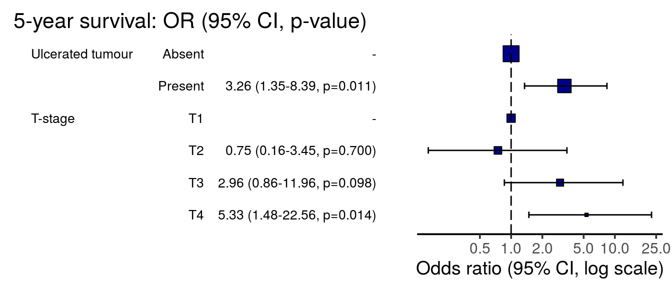
FIGURE 9.13: Odds ratio plot.
We can conclude that there is evidence of an association between tumour ulceration and 5-year survival which is independent of the tumour depth as captured by T-stage.